Synthetic Control Method
Synthetic Control Method
1. About Synthetic Control Method
Synthetic Control Method is a statistical technique used in policy evaluations. It can be deemed as an improvement for DID with matching techniques that can create homogeneous population to satisfy the parallel tendency assumption.
The basic idea is to create an artificial counterfactual outcome, called synthetic control for treatment group by doing a regression on the control group. The synthetic control is created by weighting a combination of control units that have similar pre-treatment characteristics to the treated unit. The weights are chosen to minimize the difference between the pre-treatment outcomes of the treated unit and the synthetic control.
2. Procedure of SCM
Suppose we have only one treated unit A, the factual and counterfactual outcome of it are denoted as \(Y_A\) and \(Y_A^*\). We also have \(j\) control units in the dataset, called donor pool. According to the idea of DID, we want to match the treated unit with a control unit that has parallel tendency so that we can take the outcome \(Y_c+\lambda\) as \(Y_ A^ *\). Such a unit can be hard to find as there can be multiple confounders. Nevertheless, we can find a linear combination of these control units to mimic a unit that is homogeneous to the treated unit but yield the counterfactual outcome. We called this unit a synthetic control unit.
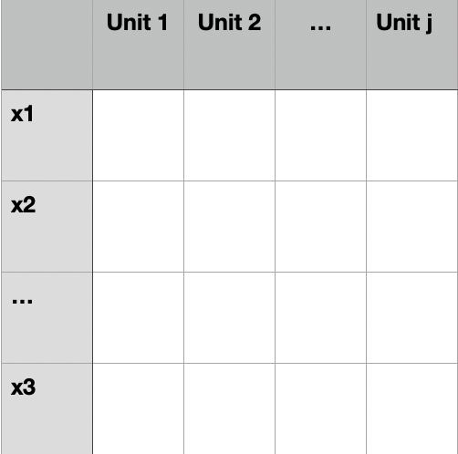
Let \(X=\{x_1,x_2...x_n\}\) denote the confounders,\(A = (T= 1,a_1,a_2,...,a_n,Y_a)\), \(S = (T= 0,s_1,s_2,...,s_n,Y_s)\) denote the treated and synthetic unit, where \(a_1...a_n,a_1...a_n\) is the pre-treatment value of confounding variables for these two unit. We can formed the input data as:
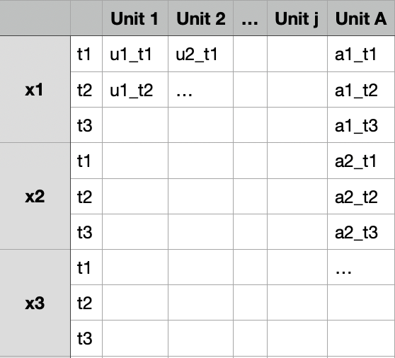
If we have time sequence data, we can stack the time dimension on the confounder dimension. The input and output data should like:
Fitting such a model would yield a series of weights \(W = (w_1,w_2,...w_j)\). Here we drop the interception in the weight vector \(w_0\). Let \(Y_C = (y_1,y_2,...y_j)\) denote the value of outcome variable for the units in the donor pool after the treatment, we estimate the counterfactual outcome as:
\[ \begin{aligned} Y^*_A &= Y_s+\lambda = W \cdot Y_C\\ \delta &=Y_A-Y_A^* = Y_A- W\cdot Y_C-\lambda\\ \lambda &= \hat{Y_A} - W\cdot \hat{Y_C} \end{aligned} \]
where \(\lambda\) is the pre-treatment difference of \(Y\) between the treated unit and the weighted sum of the donor pool.
Theoretically, we can repeat this process for each treated unit and find each of them a corresponding synthetic unit. We can then call these two group matching and calculate ATT. However, this can be very time consuming as we need to fit numerous regression model. Besides, finding the weight(conditional probability) for each pair of treated and synthetic unit can be difficult to decide. Thus, SCM are more often implemented when there is only one singles treated unit.
3. Extrapolation Problem
In the regression model of SCM, we treat the number of units as the dimension of the feature space. In practice, the number of units is often not fixed. In addition, there may be some connections between units that violate SUTVA, which can make the weight results obtained by the regression model unstable and may result in extremely large or small coefficients. We call these units with extremely large or small weights Extrapolation. Extrapolation may make the estimation results of causal effects unstable.
To solve the problem of extrapolation, we can add constraints to the optimization of linear regression. For example, we can require the weight \(w\) to be between 0 and 1, and require the sum of \(W\) to be 1. Thus, we change the optimization form of the regression problem to:
\[ \begin{aligned} &obj \ ||X_A-X_S||^2\\ &s.t. &\ 0<w_j<1 \quad \forall j \\ &\ &\sum_j^J w_j = 1 \end{aligned} \]
We can apply convex optimization tools to solve this problem.