Difference-in-differences Method

1. About Difference-in-differences

Difference-in-differences (DID) is a statistical technique to identify the causal impact of a treatment. DID methodology compares the changes in outcomes between two groups, one of which is treated with a policy intervention, and the other which isn't. The difference in the differences between the pre-treatment and post-treatment periods is the treatment effect.

Recall the idea of covariate control method in sensitivity improvement for AB Testing. Just like in A/B testing, we want to explain a portion of the variance with pre-experiment values. In causal inference, we want to explain a portion of the difference in results using the pre-difference between the treatment and control group, and remove this portion of the difference to obtain a pure causal effect of the treatment.

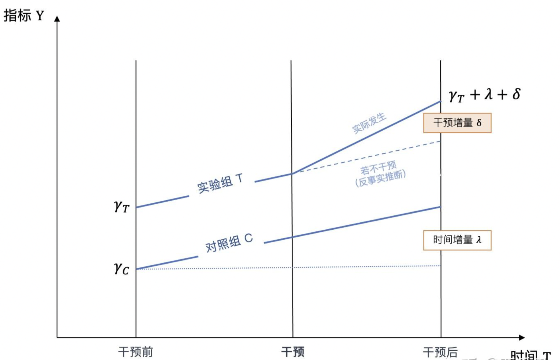
In DID, we interpret the observed \(Y_T\) and \(Y_ C\) as:

\[ Y_T = \hat{Y_T}+\lambda+\delta \]

where \(\hat{Y_ T }\) is the value of \(Y\) of the treatment group before the treatment take effect. \(\lambda\) is the increase of Y decided by time increase. Thus, we can obtain the pure causal effect \(\delta\) as:

\[ \delta = (Y_ T-Y_C) - (\hat{Y_T}-\hat{Y_C}) \]

Such an idea is simple, but it requires some assumption:

1. Linear assumption: There is a linear relationship between \(Y\) and \(T\) , that \(Y = \delta T\)
2. SUTVA: The Stable Unit Treatment Value Assumption, just like most causal inference model require
3. Parallel Trend Assumption: like demonstrated in the graph, the line representing the counterfactual outcome of treatment group should have a same tendency like observed outcome of control group. That is to say, if the treatment is not applied, the pre-difference before and after time \(t\) should remains the same.

Suppose we have an observational data that has following causal relationship:

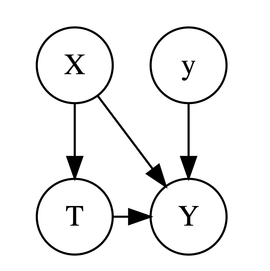
The increase by time tendency should only be brought by some exogenous variable \(y\) . Since we have some confounder \(X\) , when we we separate the samples into treatment group and control group, the distribution of \(X| T= 1\) and \(X| T= 0\) are different, this created a bias by having different \(X\) as \(X\) has a causal effect on \(Y\). Thus, when there exists confounders, the PTA is usually not satisfied.

Therefore, as DID is a simple method, we usually need to create two group that satisfies the PTA. For this reason, DID is commonly accompanied with some matching method

2. Construct Homogeneous Population

2.1 PSM

We know that after a Propensity Score Matching, we have \(T \perp \! \!\perp X \ | P\). As each unit in treatment group is matched with a unit with similar propensity score in control group, these two matched group should have same distribution of \(X\) , thus the PTA is satisfied. After a matching step of a PSM, before we weight the CATT, first we can examine the fulfillment of PTA by plotting the tendency graph of \(Y\) :

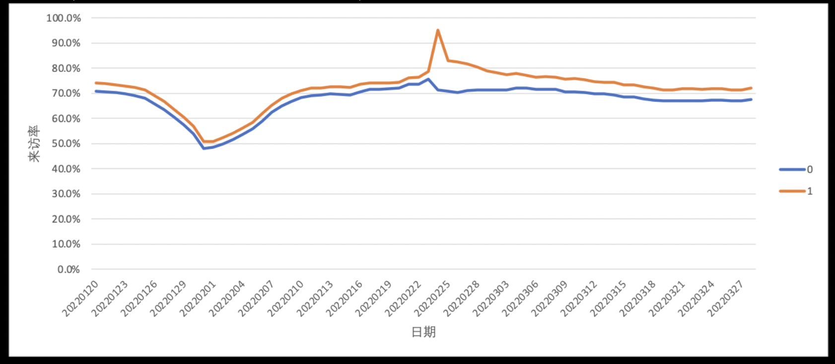
As we can see , if we found the Y of treatment and control group are parallel before treatment take effect, then the PTA is satisfied.

After the examination, we can go on with weighting and subtracting the pre-difference to obtain a more accurate pure ATT, for each unit:

\[ \tau = \frac{1}{N_T}\sum_{i \in T}\frac{1}{P_ i}(Y^T_i-Y^C_i - (\hat{Y^T_i} - \hat{Y^C_i})) \]

2.2 Difference-in-differences-in-differences(DDD)

Suppose the decision of treatment is bounded with some properties of the population, like age, gender or location. Clearly these properties will be confounders if they have an causal impact on \(Y\) .

Now suppose we have another dataset that has same distribution of \(X\) but \(T\) was never applied.

1. We use the units in this dataset that would be treated as \(T= 1\), according to their \(X\), if placed in the original dataset as a experiment group. Samely we select the control group. We conduct a DID on this dataset, and we will obtain the causal effect caused purely by \(X\) .
2. Then we conduct a DID on the original dataset, to obtained to mixed causal effect by both \(T\) and \(X\)
3. Calculate the difference between these two DID results

Such a method is called Difference-in-differences-in-differences(DDD), as we conduct two DID and compute their difference. For example, we at a state B, we want to know whether a new policy improve the health condition of elder people. In this case, the decision of \(T\) is obviously decided by whether a unit is elder. However, it’s easy to imagine that age also has a causal impact on health condition. Now suppose we have data of another state A. In this dataset of A, we select the elder people as experiment group(just for comparison, no treatment is applied), B as a control group. Conduct a DID and we will obtained the causal effect caused purely by age. Then we return to the original dataset of state B and conduct a DID, this result is contributed by both \(T\) and age, and it certain does not satisfy PTA. To fix it, we substract the portion of causal effect contributed by the age and obtain the pure effect by \(T\).

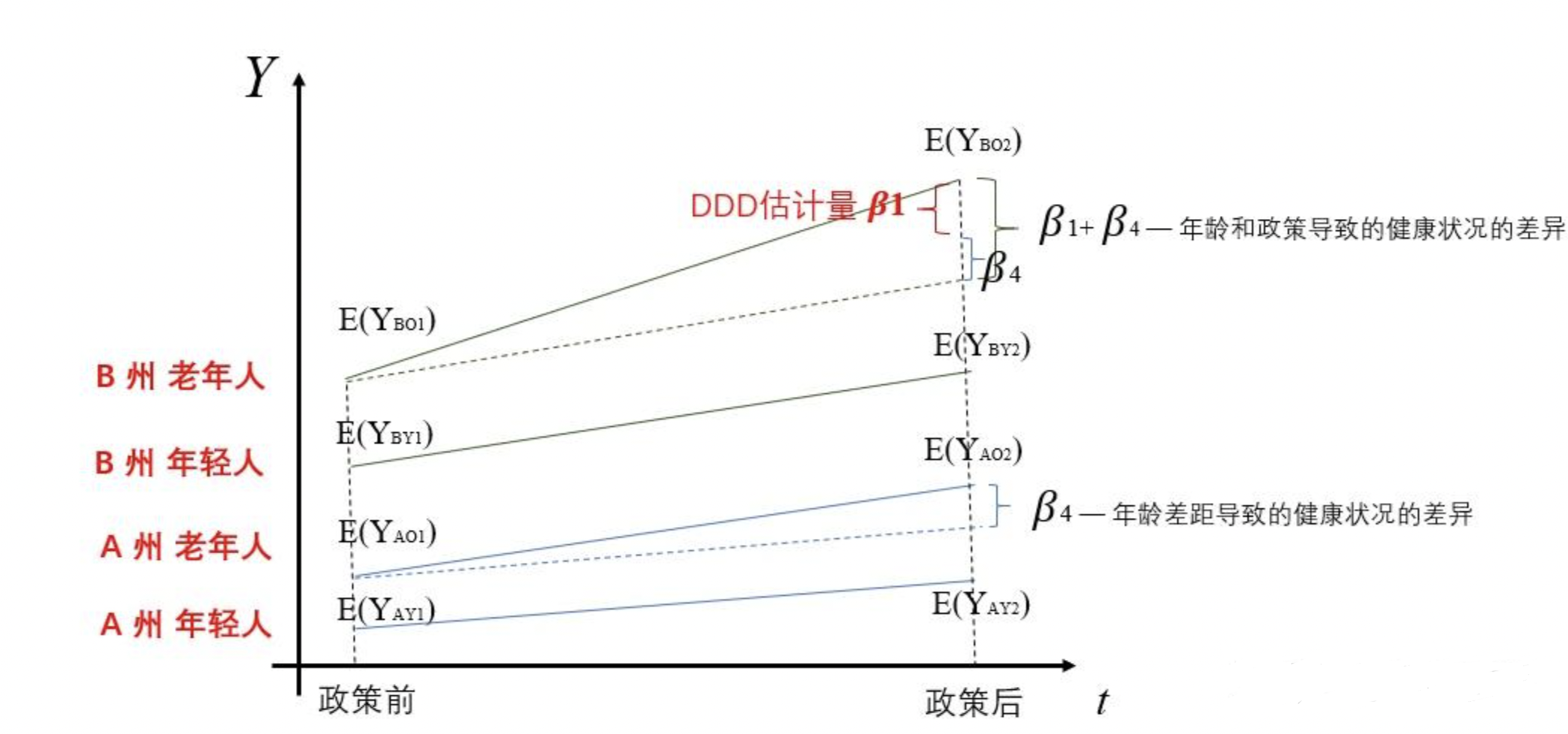
The DDD is interpretable, but in the two sub-DID, we still require PTA. That is to say, if T is decided by multiple confounders, when we condition on one of them, the PTA is still not satisfied. In this case we may need to do further sub-DID. In real application, DDD is not a frequently used method are the number of confounders are usually more than one.

2.3 Synthetic Control Method

Synthetic Control Method is a statistical technique used to estimate the causal effect of a treatment on an outcome of interest, when only one unit (e.g., state, country, company) received the treatment. The method constructs a synthetic control unit as a weighted combination of control units, which approximates the treated unit in the pre-treatment period. The weights are chosen to minimize the difference between the treated unit and the synthetic control unit in pre-treatment outcomes. The difference between the post-treatment outcome of the treated unit and the synthetic control unit is the treatment effect.

For details of SCM, refer to this article.