Propensity Score Matching

1. About Propensity Score

The propensity score matching(PSM) is a method for causal inference. Specifically, it is a method for estimating average treatment effect on treated(ATT). Recall the definition of ATT, where we have:

\[ \begin{aligned}ATT & = E[Y(1)-Y(0)|T=1]\\&= \sum_x (E[Y|X,T=1]-E[Y|X,T=0]) * P(X|T=1)\end{aligned} \]

We now introduce a new concept propensity score, it represent a unit’s propensity to select treatment \(T\) causing by factor \(X\), denoted as \(P = P(T=1|X)\). \(P\) is caused only by \(X\) and it represent the intact causal effect of \(X\) on \(T\). In a causal graph, it is demonstrated in such way:

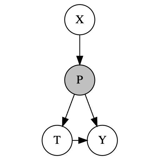
Now suppose the following assumption is satisfied:

1. There’s no unmeasured confounders(CIA).

\[ (Y(0),Y(1)) \ \perp \! \! \!\perp \ T \quad |X \]

2. As \(P\) represents all causal effects of \(X\) on \(T\) completely, when we condition on \(P\) , we can block the causal effect of \(X\) on \(T\):

\[ T \ \perp \! \! \!\perp \ X \quad |P \]

3. Common Support: \(0<P(T=1|X) <1\). When propensity score equals 0 or 1, it can excluded covariants that will directly decide \(T\) , which would make matching infeasible.

This brings us to:

\[ (Y(0),Y(1)) \ \perp \! \! \!\perp \ T \quad |P \]

With such conclusion, we have:

\[ \sum_{ P| T= 1} (E[Y|P,T=1]-E[Y|P,T=0]) * P(P|T=1) \]

We know that that in a real problem, there can exist multiple confounders and the dimension of \(X\) can be really high. The PSM conclude the affection of all confounders into a propensity score, and make it easy for computation.

2. Estimation on Propensity

The estimation of propensity score is simply a problem of probability prediction on \(P(T=1|X)\). Most probability machine learning model as well as some non-probability model can do such job, including logistic regression, naive bayes, and decision tree.

For such a machine learning model, a problem to consider is the feature selection. Features consist \(X\)should guarantee:

1. All features that simultaneously effect \(T\) and \(Y\) should be concluded, so that the CIA is fulfilled.
2. Features affected by \(T\) should be excluded. These features are invariants and should account for \(P\) .
3. The features should not cause \(P= 1\) or \(P=0\). which violate the common support assumption. From a machine learning perspective, too much features increase the variance.

Such conditions suggest we should conduct causal relationship exploring. Usually we would start with large amount of features and filtered some of them, and then conduct structural causal estimation on the remaining features to ensure condition 1 and 2 are satisfied, then fit the model again.

3. Matching

After Propensity estimation, each unit in the treatment group as well as the control group should have a propensity score in \((0,1)\). To calculate \(E[Y|P,T=1]-E[Y|P,T=0]\), we need to match unit in the treatment group with unit in control group with same or close propensity score. Common matching methods include:

Nearest Neighbors Matching

For each unit in treatment group, simply find a unit in control group with closest \(P\) . We do this with or without replacement. If without replacement, the bias would reduce but the variance would increase, as fewer samples are used in computation:

\[ \tau = \frac{1}{N_T}\sum_{i \in T}(Y^T_i-Y^C_i) \]

We can also match each unit in treatment group with multiple units in control group. In such case, we can give each neighbor a weight on causal effect according to the distance. Let \(C(i )\) denote the neighborhood of unit \(i\) in treatment group, \(\tau\) denote estimation on ATT:

\[ \tau = \frac{1}{N_T}\sum_{i \in T}(Y^T_i-\sum_{j\in C(i)}w_{ij}Y^C_j) \]

Kernel Matching

Just like what we do in many other application, we can replace NN with kernel method. Let \(G(\frac{P_j-P_i}{h})\) denote the kernel function, where \(h\) is the bandwidth:

\[ \tau = \frac{1}{N_T}\sum_{i\in T}(Y^T_i- \sum_{j \in C}\frac{G(\frac{P_j-P_i}{h})}{\sum_kG(\frac{P_k-P_i}{h})}Y^C_j) \]

For the kernel function, we can select gaussian kernel or epanechnikov kernel.

Stratification Matching

The Stratification method segment the propensity score of treated units into several section. Let \(q\) index these intervals, \(I(q)\) denote the \(q^{th}\) interval. The internal ATT is given by:

\[ \tau_q= \frac{\sum_{i \in I(q)Y^T_i}}{N_{T, q}} -\frac{\sum_{i \in I(q)Y^C_j}}{N_{C , q}} \]

The overall ATT is:

\[ \tau = \sum_q^Q\tau_q\frac{\sum_{i\in I(q)}1\{T=1\}}{\sum_{\forall i}1\{T=1\}} \]

Matching Quality Evaluation

The matching quality is basically defined on how well the propensity estimation fulfill the three assumption. The CIA is hard to test, while the common support should already been guaranteed in feature engineering, ML model optimization and matching method selection. Here we focus on examining whether \(T \ \perp \! \! \!\perp \ X \quad |P\) is satisfied. Let \(X_M^T\) denote the \(X\) of the matched treatment unit, \(X^C_M\) denote its matching group in control group. These two matched group should have same size in samples. On each matched pair, since \(P\) is conditioned, \(x^T\) and \(x^C\) should be independent, thus, \(X^T_M\ \perp \! \! \!\perp \ X_M^C\). These become to a problem of whether two variable are independent. We can use Standarized Mean Difference(SMD), covariance, correlation coefficients, Fisher’s T test, or fit a regression model for with \(T = f(X )\) and find out the \(R^ 2\) or f statistics.

4. Weighting

The difference in expectations we obtained in the matching step is biased, we need to further estimate \(P(P |T= 1)\) to estimate the unbiased ATT. A simple thought is to use the inverse of the propensity score, as larger propensity means there are less pure causal effect of \(T\to Y\) given same statistical significance. This method is called Inverse Propensity Score Weighting(IPSW):

\[ \tau = \frac{1}{N_T}\sum_{i \in T}\frac{1}{P_ i}(Y^T_i-Y^C_i) \]

We can also try probability density estimation on \(P(P|T= 1)\).

5. Sensitivity Analysis

We know that CIA requires all potential confounders included in the model. This condition difficult to satisfy. However, we can test the stability of the causal model. If the results on causla effect change greatly when we slightly add or decrease feature in confounder \(X\), then it is possible that the CIA is yet not satisfied. We can also apply skills like cross validation.