Support Vector Machine(SVM)

1. About Support Vector Machine

Support Vector Machine (SVM) is one of the most popular machine learning algorithms used for classification and regression analysis. SVM is a supervised learning algorithm that can be used for both linear and non-linear data classification. Traditional SVM assumes that the sample space is linearly separable and can be seen as a parametric model. However, with the introduction of kernel methods, SVM can infinitely expand the feature space to approximate nonlinear decision boundaries and is therefore often seen as a nonparametric model.

2. Hard-Margin SVM

2.1 Basic Idea

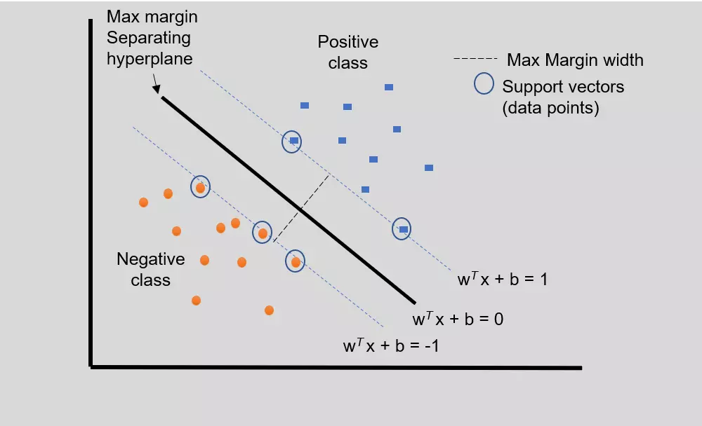
Hyperplane

SVM works by creating a hyperplane, which is a line or a series of lines that separate the data into different classes. The objective of SVM is to create a hyperplane that maximizes the margin, which is the distance between the hyperplane and the closest data points from each class. The data points that are closest to the hyperplane are called support vectors.

Suppose we have a group of data points \(\{(x_ i,y_i)\}\), where \(x\) is a vector of features \(x_i = (x_{i,1}...x_{i,m})\), \(y_i \in \{-1,1\}\) is the label of the \(i^{th}\) sample. Suppose the expression of the hyperplane in space \(x\) is \(wx+b = 0\). The case where the model correctly classified a sample is that the sample lies in the correct side of the hyperplane corresponding to its label:

\[ \left \{ \begin{aligned} &wx+b > 0 , y=1\\ &wx+b <0 , y=-1 \end{aligned}\right. \]

For all data points, we can rewrite this constraint into:

\[ y_i(wx_i+ b) > 0 \qquad \forall \ i \]

Margin

Since the margin is the distance between the hyperplane and the closest data points, the margin for each side of the hyperplane is:

\[ m = min[dist(x_i,wx+b)] = min\frac{|wx_i+b|}{||w^2||} \]

The margin is the objective we want to maximize, since \(y_i\) and \(wx_ i +b\) has same sign, we can change the objective function to:

\[ \begin{aligned} m &= min\frac{y_i(wx_i+b)}{||w^2||}\\ &=\frac{1}{||w^2||}min \ y_i(wx_i+b) \end{aligned} \]

We know there must exist some constant that \(min \ y_ i(w_i+b) = c\), since the scaler of the hyperplane does not change the results of decision of data points, we can let \(c = 1\). Now the objective function becomes \(\frac{1}{||w||}\), and now since \(min \ y_ i(w_i+b) = 1\), the constraint becomes: \(y_i(wx_i+ b) \ge 1 \ \forall \ i\). Since in optimization, we usually do minimization instead of maximization, we can transform the objective function to \(\frac{1}{2}||w ||^2\). Thus, we transform the SVM into a optimization model:

\[ \begin{aligned} min \ &\frac{||w||^2}{2}\\ s.t. \ &y_i(wx_i+ b) \ge 1 \qquad \forall i \end{aligned} \]

Suppose the optimal found are \(w^*,b^*\), then the optimal hyperplane is \(w^*x+b^*\), the final decision boundary would be \(f(x) = sign(w^*x+b^*)\)

2.2 Dual Problem of SVM

The optimization proposed in the last section is a convex optimization problem, we can solve it by solving its dual problem. By using the Lagrange multiplier method, we construct \(L(w,b,\lambda) = \frac{||w||^2}{2} +\sum_i^n\lambda_i(1-y_i(wx_i+b))\), we can write the dual form of the original problem：

\[ \begin{aligned} max \ &-\frac{1}{2}\sum_i^n\sum_j^n \lambda_i\lambda_jy_iy_jx_i\cdot x_j^T + \sum_i^n \lambda_i\\ s.t. \qquad \lambda_i &\ge 0 \qquad \forall \ i\\ \sum_i^n\lambda_iy_i &= 0 \\ \end{aligned} \]

In fact, we can prove that the primal problem and the dual problem are both QP problems, so they have strong duality and satisfy the KKT conditions:

\[ \left \{\begin{aligned} \frac{\partial L}{\partial w} = \frac{\partial L}{\partial b} = \frac{\partial L}{\partial \lambda} = 0\\ \lambda_i(1-y_i(wx_i+b))=0\\ \lambda_ i \ge 0\\ 1-y_i(wx_i+b) \le 0 \end{aligned}\right. \]

These conditions promise the following properties:

• For any points that \(wx_i+b > 1\), we have \(1-y_i(wx_i+b) < 0\), then \(\lambda_i = 0\), this point has no contribution to the optimization problem.
• For any points that \(wx_i+b = 1\), \(\lambda_i\) can be greater than 0. These points are the support vectors, they have contribution to the optimization
• \(w^ * = \sum_ i\lambda_iy_ix_i, \ b^* = y_k - \sum_i\lambda_iy_ix_i \cdot x_k^T\), where \((x_k,y_k)\) is any points that is a support vector.

These properties indicate that the optimal solution of the dual problem is sparse, and only support vectors are meaningful for optimization. As optimization progresses, the support vectors are gradually found, and the calculation of the objective function will become faster.

The mainly benefits of using dual problem is that it is easier to solve. The number of variables in the original problem depends on the feature dimensionality \(d\) of the data points. When we use kernel methods and other techniques, the number of variables to be solved is very large. However, after converting to the dual problem, the number of variables to be solved depends on the number of samples \(n\), and the calculation of inner products in the objective function can be simplified using kernel tricks. Therefore, the dual problem is often easier to solve.

3. Soft-Margin SVM

Hard-Margin SVM assumes that the dataset is linearly separable. However, in practical applications, this assumption is often not satisfied due to noise and other factors. To address this issue, Soft-Margin SVM is introduced, which allows for some misclassified points to exist between support vectors. It uses the idea of regularization, relaxes the constraints of the optimization problem, and penalizes misclassified points as a penalty term in the objective function:

\[ min\ \frac{1}{2}||w||^2 + \sum_iloss(x_i) \]

If we directly use the number of misclassified points as the penalty term, then \(loss(x_i)\) will be discontinuous with respect to \(w\). Therefore, we define:

\[ \xi_i = loss(x_i) = \left \{ \begin{aligned} &0 \ &y_i(wx_i+b) \ge 1\\ &1-y_i(wx_i+b) \ &y_i(wx_i+b) < 1\\ \end{aligned}\right. \]

we can rewrite it into:

\[ \xi_i = max[0,1-y_i(wx_i+b)] \]

We can use a parameter C in \([0,\infty)\) to control the extent of penalty. The objective function and constraints now become:

\[ min\ \frac{1}{2}||w||^2 + C\sum_i\xi_i \]

\[ \begin{aligned} min\ &\frac{1}{2}||w||^2 + C\sum_i\xi_i\\ s.t. \ &y_i(wx_i+ b) \ge 1-\xi_ i \qquad \forall i \end{aligned} \]

This function is also called hinge loss

4. Kernel Method in SVM

4.1 Kernel Method

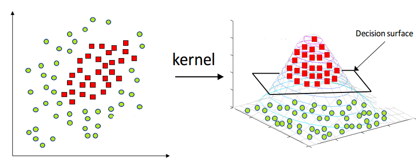
SVM assumes the dataset is linear separable. However, in most application it is not the case. If there’s only slight non-linearity in the dataset, we can use soft margin SVM to solve problem. However , when the dataset is strictly not linear separable, we need to introduce kernel method. Kernel Method is a way to solve nonlinear problems by mapping the original data to a higher-dimensional space where the problem becomes linearly separable.

Suppose the original feature space is \(d = (x_1,x_2)\), let \(\phi(x)\) denote a high dimensional mapping that \(\phi(x) = (x_1,x_2,(x_1-x_2)^2)\)), then we would get such effect:

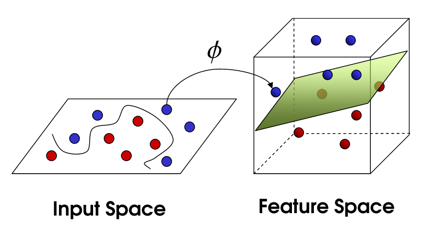
Note that every dimension of the new space can be a non-linear transformation(usually non-linear), we do have to retain the original feature x. By using kernel methods, SVM can handle nonlinear problems and provide high accuracy for a wide range of applications.

4.2 Kernel Function

By transforming SVM into a dual problem, we make the variables to be optimized dependent on the number of samples \(n\), but when calculating the objective function, we still need to compute the dot product \(\phi(x_i) \cdot \phi(x_j^T)\). When using kernel tricks, if \(x\) is mapped to a high-dimensional space, computing the dot product can still be very time-consuming.

Now, let us assume that a function satisfies the following property: suppose \(x_i,x_j\) are two data points in the original space, and \(\phi(x)\) can map data points in the original space to a high-dimensional space \(z\). If there exists a function \(K\) such that:

\[ K(x_i,x_j) = \phi(x_i)\phi(x_j)^T \]

So we call the function \(K(x_i,x_j)\) a positive definite kernel function. Usually, the kernel function is what we use in practical applications, so we simply refer to it as the kernel function. The kernel function can transform the calculation of the vector inner product \(\phi(x_i) \cdot \phi(x_j^T)\) in the dual problem objective function into a function calculation \(K(x_i,x_j)\). This greatly simplifies the computational complexity of dual problem optimization, making it no longer dependent on the dimension of \(\phi(x)\), but rather dependent on the number of samples. We know that the inner product of two vectors represents the angle between the two vectors in space, that is, the similarity of the two vectors. Therefore, the kernel function actually represents the similarity of two samples in some high-dimensional space.

To determine whether a function is a positive definite kernel function, we mainly use the two properties of positive definite kernel functions.

• Symmetry：\(K(x_ i, x_j) = K(x_j,x_i)\)
• Positivity：for any \(n\) points \((x_1,…x_n)\), the gram matrix is a positive semi-definite matrix

\[ G = \begin{bmatrix} K(x_1,x_1) & ... &K(x_1,x_n)\\ ... & K(x_i,x_j) &...\\ K(x_n,x_1) &... &K(x_n,x_n) \end{bmatrix} \]

Common kernel function includes:

• Linear Kernel: \(K(x_i,x_j) = x_i \cdot x_j\)
• Polynomial Kernel: \(K(x_i,x_j) = (ax_i \cdot x_j + b)^d\)
• Gaussian RBF Kernel: \(K(x_i,x_j) = \exp(-\frac{||x_i-x_j||^2}{2\sigma^2}) = \exp(-\gamma||x_i-x_j||^2)\),
• Sigmoid Kernel: \(K(x_i,x_j) = tanh(\gamma x_i\cdot x_j+r)\)

where \(\gamma\) represents an adjustable hyper-parameter.

For SVMs that use kernel tricks, the final decision boundary is:

\[ f(x) = sign(\sum_i^n\lambda_i y_i K(x,x_i)+b ) \]

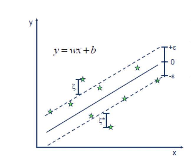
5. Support Vector Regression

SVM can also be used for regression analysis, called Support Vector Regression (SVR). SVR is particularly useful for datasets with a large number of features and complex nonlinear relationships between the features and the target variable, as it can apply kernel method as well.

Suppose we want to regress a linear hyperplane \(y = wx+ b\) . Now we decide we can tolerate some error if the distance between the true data point \(y_i\) and the prediction \(\hat{y_i }\) if they are close enough. Then the modified MAE loss function is:

\[ \xi_i = loss(x_i) = \left \{ \begin{aligned} &0 \ &|y_i-\hat{y_i}| \le \epsilon\\ &|y_i-\hat{y_i}| \ &|y_i-\hat{y_i}| > \epsilon\\ \end{aligned}\right. \]

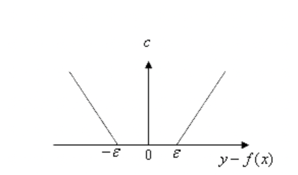
We call the region within \(\epsilon\) distance from the hyperplane the \(\epsilon\)-insensitivity zone. Ideally, we want all data points to fall within this zone (constraint). During training, we can treat the points outside of this region as penalty terms in the optimization process (slack variables). We add a regularization term \(\frac{1}{2}||\omega||^2\) in the loss function, the training of the regression model can then be written as:

\[ \begin{aligned} min\ &\frac{1}{2}||w||^2 + C\sum_i\xi_i\\ s.t. \ &|y_ i - (wx_i+ b)| \le \epsilon +\xi_ i \qquad \forall i \end{aligned} \]

We found that the optimization problem is very similar to the form of Soft Margin SVM, and we can use the same techniques, kernel functions, dual problem solving methods, etc. to solve this problem. We call such a model a Support Vector Regressor（SVR）, the data points lie out of the zone is the support vectors.

By discussing different cases, removing absolute value signs, we can transform the above problem into a convex problem. For each data point \(x_i\), we introduce two slack variables \(\xi_i^+\) and \(\xi_i^-\), which represent the distance from the point to the upper boundary of the \(\epsilon\)-insensitive zone and the distance from the point to the lower boundary of the \(\epsilon\)-insensitive zone, respectively. If a data point is not within the \(\epsilon\)-insensitive zone, then it can only be either above or below the zone, and thus at most one of \(\xi_i^+\) and \(\xi_i^-\) can be non-zero for the same data point. We can then formulate the optimization problem as follows:

\[ \begin{aligned} min\ \frac{1}{2}||w||^2 + C\sum_i（\xi_i）\\ s.t. \ y_ i - (wx_i+ b) &\le \epsilon +\xi_i^+ \qquad \forall i\\ \ (wx_i+ b)-y_ i &\le \epsilon +\xi_i^- \qquad \forall i\\ \xi_ i^+ >0, \xi_i^- >0 \end{aligned} \]

We can also derive the dual form of SVR using the Lagrange multiplier method, which is not listed here. Through the dual form, the optimal hyperplane can be obtained as:

$$ \[\begin{aligned} f(x) &= \sum_i(\lambda_i^+-\lambda_i^-)x\cdot x_i^T +b^*\\ \end{aligned}\]

$$

\[ b^* = \left\{\begin{aligned} -\sum_i(\lambda_i^+-\lambda_i^-)x_i \cdot x_k^T+\epsilon+y_k, \ 0\le\lambda_k^+\le C\\ -\sum_i(\lambda_i^+-\lambda_i^-)x_i \cdot x_k^T-\epsilon+y_k, \ 0\le\lambda_k^-\le C\\ \end{aligned}\right. \]

where \((x_ k, y_ k )\) is the closest support vector.

When applying kernel method, the optimal hyperplane is:

$$ \[\begin{aligned} f(x) &= \sum_i(\lambda_i^+-\lambda_i^-)K(x,x_i) +b^*\\ \end{aligned}\]

$$