Basics of Markov Chain

1. About Markov Chain

Markov Chain is a mathematical model used to describe a system's behavior over time, where the future state of the system depends only on its current state. It is a stochastic process that is widely used in various fields such as physics, economics, and computer science.

A Markov Chain is a sequence of random variables, where each variable represents the state of the system at a specific time. The probability of transitioning from one state to another is based only on the current state of the system, and not on the past states.

Let \(X_ n\) denote a be a stochastic process that takes on finite possible values \(\{0,1,...m \}\). For all \(i, j , n\), if we have:

\[ P\{X_{n+1} = j | X_n = i, X_{n-1} = i_{n-1},...X_0 = i_0\} = P\{X_{n+1} = j | X_n = i\} \]

Then we said this random process has Markov Property. We can \(P\{X_{n+1} = j | X_n = i\}\) the one-step transition probability from state \(i\) to state \(j\) , denoted as \(P_ {ij}\).

2. Discrete Time Markov Chain

2.1 Transition Matrix and Transition Diagram

We can expressed the one-step transition probability among states of a markov chain in 2 ways.

Transition Probability Matrix

We define the one-step transition probability matrix as:

\[ P = \begin{bmatrix} P_{0,0 } & P_ {01}&... & P_{0m}\\ P_{10} & P_{11} & ...\\ ... & ... &...\\ P_{m0} & P_{11} & ... & P_{mm}\\ \end{bmatrix} \]

where each element is a one-step transition probability from the state of the row index to the state of the column index. The sum of each row \(\sum_jP_{ij} =1\) .

Let \(P^n_{ij} = P\{X_{n+k} = j |X_k = i\}\). We call this the n-step probability from state \(i\) to state \(j\). According to the Chapman-Kolmogorov equations, we can deduce that:

\[ \begin{aligned} P^{n+m}_{ij} & = P\{X_{n+m} = j | X_0 = i\}\\ & = \sum^\infty_0P\{X_{n+m}\ = j,X_n = k | X_0 = i\} \\ & = \sum^\infty_0P\{X_{n+m}\ = j| X_n = k , X_0 = i\}P\{ X_n = k| X_0 = i\} \\ & = \sum^\infty_0 P^m_{kj}P^n_{ik} \end{aligned} \]

Let \(P^{(n )}\) denote the n-step transition probability matrix. According to this deduction, we can further obtain that:

$$ \[\begin{aligned} P ^{(n+m)} &= P^{(n)} \cdot P^{(m)}\\ P^{(2)} &= P \cdot P\\ P^{(n)} &=P^{(n- 1)} \cdot P = P^ n \end{aligned}\]

$$

Transition Diagram

The transition probabilities can also be expressed in a transition diagram

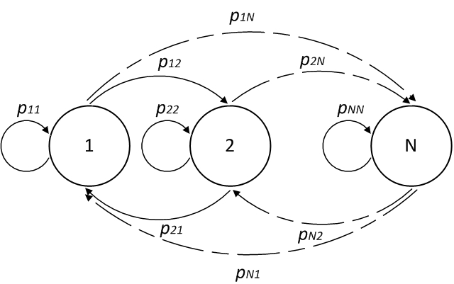
The circles in the graph represent states.The directed arrow in the graph represent the one-step transition.

2.2 Classification of States

Communicate

State \(j\) is said to be accessible from state \(i\) if \(P_{ij}^n > 0\) for some \(n\) . In other word, start from state \(i\) , it is possible to ever enter state \(j\) . If two state are accessible from each other, we say these two states communicate. If \(i\) communicate with \(j\) , j communicate with \(k\) , then \(i\) communicate with \(k\) . We call a group of states \(\{i_ 0,i_ 1,...\}\) a class if every pair of states in the class communicates. If any two states of a markov chain communicates, then there is only one class of states. In this case, we call the markov chain irreducible.

Recurrent and Transient

We said a state \(i\) is recurrent if \(\sum^ \infty _{n= 1} P^n_{ii} = \infty\), or is transient if \(\sum^ \infty _{n= 1} P^n_{ii} < \infty\). This can be more clearly understood from a transition diagram:

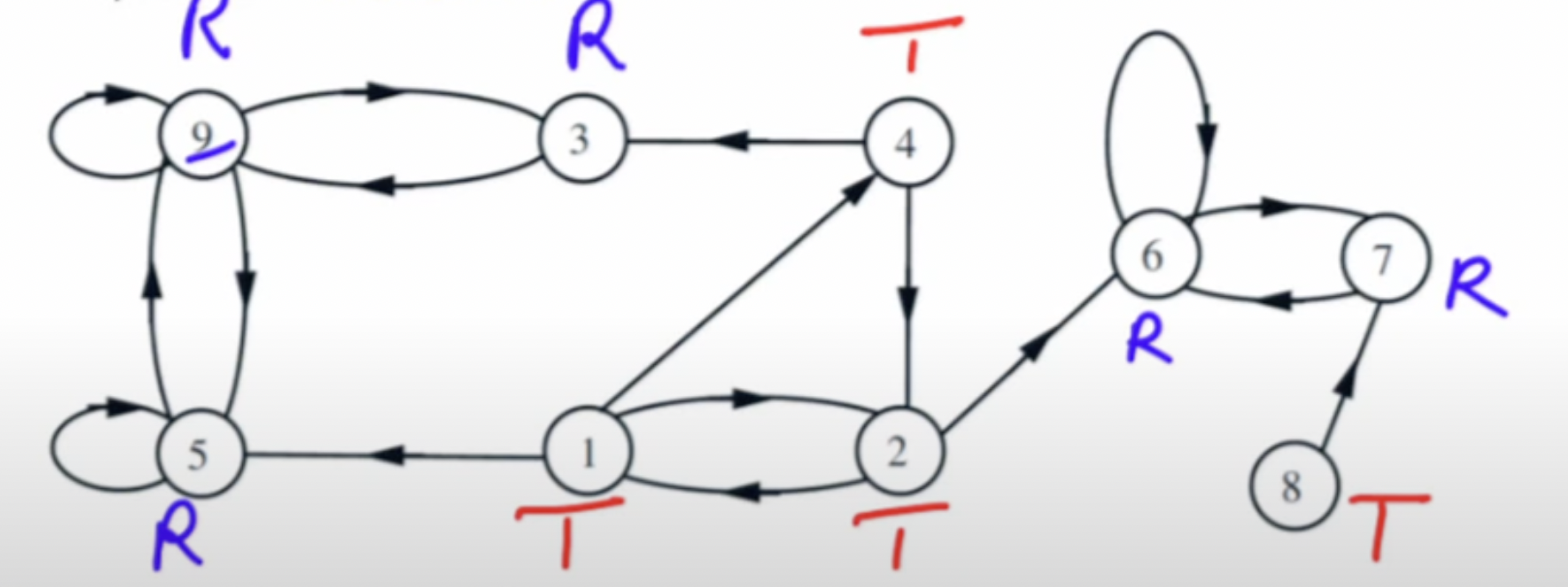
We say state \(i\) is recurrent if, starting from state \(i\) , wherever you go to, you can always find a way back to \(i\).

On the contrary, we sat state \(i\) is transient if, starting from state \(i\), if you go to some where, you can never find a way back to \(i\) .

• If state \(i\) is recurrent, and state i communicates with state \(j\) , then state \(j\) is recurrent.
• If state \(i\) is transient, and state i communicates with state \(j\) , then state \(j\) is transient.
• Recurrent and transient are class properties. If one element if the class is recurrent or transient, then all elements in that class are recurrent or transient as well
• At least one state in a Markov Chain should be recurrent
• Let \(\mu_ {ii }\) denote the expectation of steps it takes from \(i\) back to \(i\). If \(\mu_{ii } > 0\), we call it positive recurrent, if \(\mu_ {ii} = 0\), we call it zero recurrent.
• If state \(i\) is transient, then the number of times the process will reenter \(i\) follows a geometric distribution \(Geo(1-f_{ii })\), where \(f_{ii }\) is the probability that the process will ever reenter \(j\) from \(j\) .

Periodical

For a state \(i\), let \(d\) denote the Greatest Common Divisor of a collection of n that \(P^n_{ii} > 0\) (\(d = 0\) if the collection is empty ). If \(d > 1\), then we said this state is periodical. For example, a state is only possible to reenter itself when the step \(n = 2,4,6,8,...\). The greatest common divisor is 2. which makes this state periodical. If a state is:

1. aperiodic
2. positive recurrent

we call this state ergodic. If all states in an irreducible markov chain is ergodic, then we call this markov chain a ergodic chain

2.3 Stationary Distribution and Balance Equations

Consider a markov chain go through infinite steps. Under some condition, we would find that:

\[ \lim _{n \to \infty}P^{(n)} = \begin{bmatrix} \pi(0) & \pi(1)&... & \pi(m)\\ \pi(0) & \pi(1)&... & \pi(m)\\ ... & ... &...\\ \pi(0) & \pi(1)&... & \pi(m)\\ \end{bmatrix} \]

If this limitation does exists, we call the markov chain reach a stationary distribution. The limitation \(\pi(i )\) is called the long-run proportion or stationary probability of state \(i\) . \(\sum_i^m \pi(i) = 1\).

The condition of being able to reach stationary distribution is complex, but basically, a markov chain will eventually converge if it satisfies:

1. irreducible
2. all states are aperiodic

A important property of stationary markov chain is that, for each state, the “flow- in” equals the “flowout”. For example, in such a transition diagram:

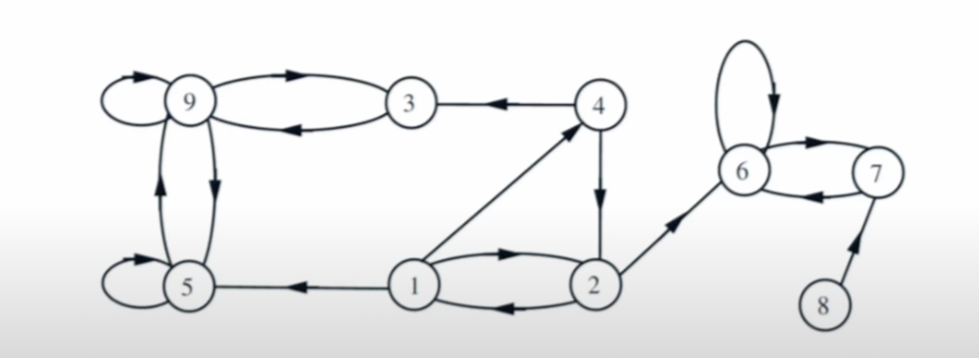
for state 9, it should have:

\[ (P_{99}+P_{93}+P_{95})\pi_9 = P_{59}\pi_5+P_{39}\pi_3 \]

For a markov chain, \(\sum_ jP_ {ij} =1\), thus:

\[ \pi_9 = P_{59}\pi_5+P_{39}\pi_3 \]

Specifically, for a markov chain reach stationary distribution, let \(\pi = (\pi_1,\pi_ 2,...\pi_ m)\) , P denote the one-step transition probability matrix, we should have:

\[ \pi = \pi \cdot P \]

Thus, we can find the long-run proportion by solving a system of equations. We call this system of equations the stationary balance equations.

Specifically, if the stationary distribution of a markov chain does not change when we reverse the time order, we call this markov chain time reversible. In this case we have:

\[ \begin{aligned} \pi_i P_{ij} &= \pi_i P_{ji}\\ \pi \cdot P &= \pi \cdot P^ T \end{aligned} \]

It can be proven that a time reversible markov chain has to be able to reach stationary distribution.

If a markov chain has transient states, it is not irreducible and does not necessarily have a stationary distribution. In such case, we can still calculate the mean time spent in transient states. Such a mean is different given different start point. Since it is impossible to enter transient state from recurrent state, the start point can only be transient states.

Let \(T = \{0,1,2,...t \}\) denote the collection of all transient states. \(P_T\) denote the one-step probability matrix consists only of these states. Note here the row sums of \(P_T\) can be less then 1. Let \(s_{ij}\) denote the mean number of steps that the process stay in \(j\) if it starts from \(i\). Let:

\[ S = \begin{bmatrix} s_{01} & s_{02}&... & s_{0m}\\ s_{11} & s_{12}&... & s_{1m}\\ ... & ... &...\\ s_{m1} & s_{m2}&... & s_{mm}\\ \end{bmatrix} \]

With proofing omitted, we can obtained:

\[ S = (I - P_T) \]

3. Continuous Time Markov Chain

3.1 Transition Rate

We said a random process is a Continuous Time Markov Chain if for all moments and states, we have:

\[ P\{ X_{s+t} = j | X_1 = i_1,...X_s= i_s\} = P\{ X_{s+ t} = j|X_s = i \} \]

If this probability is independent to \(s\) , we say this markov chain has a stationary transition probability, denoted as \(P_{ij}(t )\). We can such markov chain a Time-homogeneous Markov Chain. For example, the Poisson Process is a time-homogeneous CTMC.

In a continuous time Markov chain, the transition times \(t\) between states are exponentially distributed. After \(t\) , the process leaves \(i\) and enter state \(j\) with a probability \(P_ {ij }(t )\), where \(\sum_jP_{ij}(t ) =1\), \(P_{ii}(t ) =0\). The probability of transitioning from state \(i\) to state \(j\) in a small time interval \(\Delta t\) is given by \(P_ {ij}(\Delta t) = q_{ij}\Delta t\), where \(q_{ij}\) is the rate, or to say, the probability of transition from state \(i\) to state \(j\) in a unit time. According to Chapman-Kolmogorov equations, we can define \(q_{ij}\) as:

$$ \[\begin{aligned} q_{ij} &= \lim_{\Delta t \to 0} \frac{P_{ij}(\Delta t)}{\Delta t} \qquad i \ne j\\ q_{ii} &= \lim_{\Delta t \to 0} \frac{P_{ii}(\Delta t) - 1}{\Delta t} \end{aligned}\]

$$

We can then obtain the transition rate matrix of a CTMC:

\[ Q = \begin{bmatrix} q_{00} & q_{01}&... & q_{0m}\\ q_{11} & q_{12}&... & q_{1m}\\ ... & ... &...\\ q_{m1} & q_{m2}&... & q_{mm}\\ \end{bmatrix} \]

The diagonal entries of the rate matrix \(Q\) are negative so that the row sums equal zero:

\[ q_{ii} = \sum_{j \ne i} q_{ij} \]

In other would, the entry \(q_{ii}\) actually represents the opposite number of “flow-out”. This Matrix \(Q\) has same meaning as the one-step transition probability matrix in a DTMC, and the matrix of \(P(t )\) has the same meaning as the matrix \(P^{(n )}\) in DTMC.

3.2 Stationary Balance Equations

The condition that a CTMC can reach stationary distribution is simply irreducible.

Back to the definition of transition rate, we can deduce the following equations:

\[ P'_{ij}(t) = \sum_{k \ne j}q_{kj}P_{ik(t)} - v_iP_{ij}(t) \]

\[ P'_{ij}(t) = \sum_{k \ne i }q_{ik}P_{kj(t)} - v_iP_{ij}(t) \]

where \(v_i = \sum_{j \ne i} q_{ij}\), representing the total “flow-out” amount of state \(i\).

These two equations are called Kolmogorov’s Forward Equation and Kolmogorov’s Backward Equation.

Like DTMC, we define the stationary probability as:

\[ \lim_{t \to \infty} \begin{bmatrix} p_{00}(t) & p_{01}(t)&... & P_{0m}(t)\\ p_{11}(t) & p_{12}(t)&... & q_{1m}(t)\\ ... & ... &...\\ p_{m1}(t) & p_{m2}(t)&... & p_{mm}(t)\\ \end{bmatrix} = \begin{bmatrix} \pi(0) & \pi(1)&... & \pi(m)\\ \pi(0) & \pi(1)&... & \pi(m)\\ ... & ... &...\\ \pi(0) & \pi(1)&... & \pi(m)\\ \end{bmatrix} \]

where \(\pi_i\) standards for the limitation probability, or long-run proportion of state \(i\). Let \(\pi = (\pi_0,\pi_1,...\pi_m)\). Since the limitation probability is a constant, \(\frac{dP(t)}{dt} =0\) , we can then transform the Kolmogorov ‘s equations into:

\[ 0= \pi \cdot Q \]

\[ 0= Q \cdot \pi \]

These give the stationary balance equations of a CTMC.