Common Dimension Reduction Methods

1. About Dimension Reduction

In the world of data analysis, it is common to encounter datasets with a large number of variables or features. While each variable can provide valuable information, the sheer volume of data can make analysis difficult and time-consuming. This is where dimension reduction comes in as a powerful tool to simplify complex data analysis. Dimension reduction is a statistical technique that reduces the number of variables in a dataset while retaining as much of the original information as possible.

There are two types of dimension reduction. The first involves directly extracting a subset from the original feature space. The second involves mapping the high-dimensional data into a low-dimensional feature space. We mainly focus on the second method. Therefore, in this article, the term "dimensionality reduction" specifically refers to mapping features of high-dimensional space to low-dimensional space.

2. Principal Component Analysis(PCA)

One popular dimension reduction method is Principal Component Analysis (PCA). This method transforms a large number of variables into a smaller set of uncorrelated variables known as principal components. These principal components are linear combinations of the original variables and are sorted in order of the amount of variance they explain in the data. By selecting the first few principal components, we can effectively reduce the dimensionality of the data without losing too much information.

2.1 Variance Maximization Theory

The PCA algorithm has multiple theoretical explanation. Here we adopt the Variance Maximization Theory. We know that in signal processing, signal usually has variance than noise, the Variance Maximization Theory believes variance contains information. For dimension reduction, our task is to map high dimension space data points into low dimension space with minimum information loss, in other word, maximum variance.

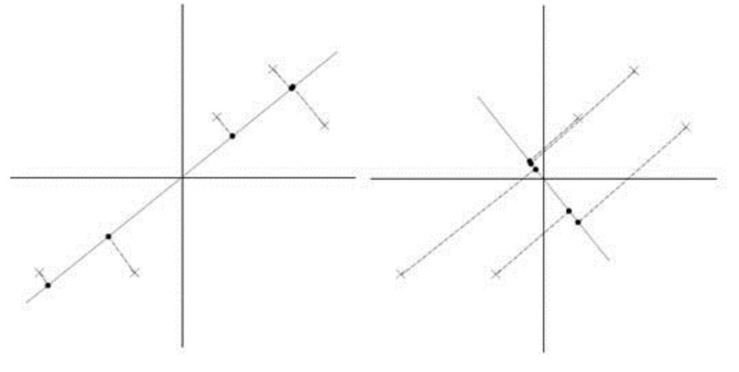
For example, in the graph above, we want to map some two-dimension data points into a one-dimension space(a line). In this case, the left graph is a better mapping than the right one, as it produce higher variance after mapping.

Now we inspect the mapping process:

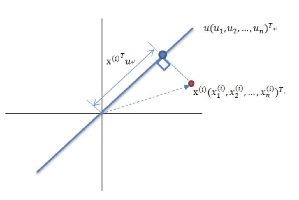
We know that if we map a vector to a direction, the magnitude of \(x\) after the transformation is \(d = |x| |u| cos\theta=x \cdot u^T\) \(d\). If the linear space represented by \(x\) is standardized (with mean 0 in every dimension and no dimensional differences in scale), then the transformed space remains standardized. Let \(\mu _j\) denote the mean of the \(j^ {th }\)dimension after transformation, \(\mu_ j = 0\), then the Variance on that dimension is \(V_ j = \frac{1 }{n}\sum_i^n(d_{i,j} - \mu_j)^2 = \frac{1 }{n}\sum_i^n(d_{i,j})^2\), where \(n\) is the number of samples, \(d_{i,j}\) is the length of mapped vectors on dimension \(j\) of the \(i^{th }\) sample.

As the Variance Maximization Theory suggests, we want the to find a space(a group of vectors that) allows maximum variance in all all dimensions. However, if the these vectors are highly correlated, then each pair of dimensions would have high covariance. It can be imagined that if we find a single direction that maximizes the variance (magnitude) of the mapping of the original x in that direction, then finding some directions "almost coincident" with that direction can achieve maximum variance. But this group of vectors is meaningless because there is too much redundant information between them, and each vector represents features that are almost identical in meaning. Therefore, on the basis of maximizing the variance as much as possible, it is also necessary to assume a constraint that makes the covariance as small as possible. According to this, we obtained the main idea of PCA: to find a space that:

1. has lower dimension then the original feature space
2. has as much total variance as possible
3. is orthogonal, that the covariance of each two dimensions is 0

We know that the covariance of two variable is given by:

\[ Cov[X,Y] = E[(X-E[X])(Y-E[Y])] \]

In a standardized space, the expectation of any dimension is 0, thus, for two feature:

\[ Cov[X,Y] = E[XY] = \frac{1}{n-1}\sum_i^n(X_i,Y_i) \]

We can then obtained the covariance matrix:

\[ corr = \frac{1}{n-1}\begin{bmatrix} Cov[X_1,X_1..] & Cov[X_1,X_2] & ... \\ Cov[X_2,X_1] & ... & ... \\ ... & ... & Cov[X_n,X_n] \\ \end{bmatrix} = \frac{1}{n-1}X^TX \]

The diagonal of the covariance matrix represent the variance of the feature, other elements represent the covariance between a pair of dimension.

Back to our objective, we want the covariances of the mapped space to be 0, will we want the variances of the space remain as high as possible. Let X denote the original space(dataset), P denote the mapping vectors, \(Y = XP\) denote the new space after mapping. Let \(D\) denote the covariance matrix of Y. If D is diagonal matrix, that all elements not on the diagonal are 0, while the elements on the diagonal remains positive value or 0, we can claim that we found a P that fit our PCA optimization objective. Then we can select the top k dimensions sorted by magnitude of mapped vectors(Variance), and believe these dimensions contain most of the information of the original space and call them Principal Components.

But how can we find the desired \(D\)? Since the \(D\) we described above is also a standardized space, we can write this covariance matrix into:

\[ \begin{aligned} D &= \frac {1}{n-1} Y^TY \\ & = \frac {1}{n-1}(XP)^T(XP)\\ & = P^T(\frac {1}{n-1}X^TX)P \end{aligned} \]

Now we can find that the part \(\frac {1}{n-1}X^TX\) happen to be the covariance matrix of the original space, as it is also a standardized space. We denote this covariance matrix as \(C\). Suppose vectors in P we want to find can be normalized as a unit vectors. In this case, the P is a unitary matrix, that \(P^T = P^{-1}\)

\[ C = PDP^{-1} \]

Since D is a diagonal matrix, we can find that this process is actually a eigenvalue decomposition of the original covariance matrix \(C\). In other word, the P we want to find is the unit eigenvectors of C.

2.2 Steps of PCA

With the analysis in 2.1, we can conclude the procedures of implementing a PCA algorithm:

1. Applied Standardization on the original dataset’s feature space. Note that this assume the feature space is normal distributed. If that is not the case, we should consider normalization transformation
2. Calculate the Covariance Matrix C
3. Decompose \(C = PDP^ T\) to obtain eigenvectors matrix \(P\)
4. sort the diagonal of \(D\) (Variance), select top \(k\) values, \(k\) is a hyperparameter
5. Based on the selected feature values, find the corresponding k feature vectors and form a matrix \(P_{m \times k}\)
6. \(Y_{n\times k} = X_{n\times m}P_{m\times k}\). \(Y\) is the transformed data.

2.3 SVD Realization of PCA

We know that in Singular Value Decomposition, the way we obtain the singular matrix \(U\) and \(V\) is to conduct eigenvalue decomposition on \(A^T A\) and \(A^TA\). As discussed above, these two matrix are equivalent to the covariance matrix for standardized space. That is to say, SVD can replace eigenvalue decomposition to realize the thought of PCA. For a dataset \(X_{n\times m }\), according to SVD:

\[ X_{n\times m} = U_{n\times n}\Sigma_{n \times m} V_{m \times m}^T \]

If we consider column space as the feature space:

\[ X_{n \times m}V_{m \times m} = U_{n\times n}\Sigma_{n \times m} \]

This process maps n data points onto a set of m-dimensional orthogonal basis, and the size of each direction is determined by the elements on the corresponding main diagonal of \(\Sigma\). Conversely, if the row space is defined as the feature space:

\[ X_{m \times n}^TU_{n \times n} = V_{m\times m}\Sigma_{m \times n}^T \]

At this point, we represent mapping m data points onto a set of n-dimensional orthogonal bases. Singular values remain elements on \(\Sigma\). Note that when \(m < n\), we can only find m singular values, but this does not affect our ability to compress n into smaller numbers according to the order of singular values.

After selecting the feature space, similar to PCA, we can sort the singular values and select the top k singular values and their corresponding singular vector matrix. For example, if we select the column space as the feature space:

\[ Y_{n,k} = X_{n \times m}V_{m \times k} \]

In real application, many package use SVD to realize PCA, this is because comparing to eigenvalue decomposition, SVD has some advantages:

1. In some package, the SVD process can avoid the calculation of covariance matrix \(\frac{1}{n}X^TX\) , which is very time consuming when the dimension of feature is high
2. SVD can do dimension reduction on both row space and column space. This is useful when the features are associated with both rows and columns. For example, in graph compression, both rows and columns are pixels, or in recommendation system, both user and item are considered feature.

3. T-Distributed Stochastic Neighbor Embedding

Another dimension reduction method is t-Distributed Stochastic Neighbor Embedding (t-SNE). Unlike PCA, t-SNE is a non-linear method that is particularly useful for visualizing high-dimensional data. t-SNE maps high-dimensional data points to a low-dimensional space while preserving the relative distance between them. This makes it possible to visualize clusters of similar data points that may not be apparent in the original high-dimensional space.

3.1 SNE

The basic idea if SNE is to construct a conditional probability distribution that describe the similarity(distance). If two data points are close in the original space, in other word, one point is very possible to be found near another point, then the same situation should happen in the low dimension space after mapping.

Given a data point i, Let \(p_{j|i}\) denote the probability that we can find j in the neighborhood of i in the high dimension space. We can calculate \(p_{j|i}\) with the euclidean distance:

\[ p_{j|i} = \frac{-e^{\frac{||x_j - x_i||^2}{2\sigma^2_i}}}{\sum_{k \ne i} e^{-\frac{||x_k - x_i||^2}{2\sigma^2_i}}} \]

Note that \(\sigma_i\) is a manually defined parameter, and it should be different for different points i. Specifically, \(p_{j|j } = 0\)

Let \(q_{j|i}\) denote the same probability in the low dimension space. In the low dimension space, let \(\sigma_i\) for any i be \(\frac{ 1}{\sqrt{2}}\).

\[ q_{j|i} = \frac{-e^{||y_j - y_i||^2}}{\sum_{k \ne i} e^{-||y_k - y_i||^2}} \]

As the idea of SNE suggests, \(p_{j|i}\) and \(q_{j|i}\) should be two similar distribution. We can thus use the KL divergence(refer to this article) to measure the similarity.

\[ C = \sum_iKL(p_{j|i}q_{j|i}) = \sum_i\sum_jp_{j|i}log\frac{p_{j|i}}{q_{j|i}} \]

To find a group of \(\sigma_i\), the SNE introduce the concept of perplexity.

Larger \(\sigma _i\) would enlarge the neighborhood of point i, which would include more other point in the interval and hence increase the entropy. Let \(P_i\) denote the probability distribution of \(p_{j| i}\) given i, \(H(P_ i)\) denote the entropy of distribution \(P_i\) . Define Perplexity as:

\[ Perp( i) = 2^{H(P_i)} \]

This hyper parameter, perplexity, is decided by the number of points in the neighborhood for any point i. SNE would adjust \(\sigma_i\) for each i to let the perplexity calculated from data point i approximate the preset perplexity by the user. Choosing 2 as the base is because SNE commonly uses binary search to search for conditions \(\sigma_i\) .

With these set, we can optimize the loss, which is the KL divergence and update the lower dimension mapping data points using momentum optimization

\[ Y^{(t)} = Y^ {(t- 1)} + \eta \frac{\partial C}{\partial Y} +\alpha(t)(Y^{(t-1)} - Y^{(t-2)}) \]

3.2 Improvement of SNE

Symmetric SNE

KL divergence is asymmetric. Asymmetry makes computing the derivative of KL divergence very time-consuming。 One approach is to modify the conditional probability to joint probability, so that \(p_{i,j} = p_{j,i}\), which can simplify the calculation:

\[ p_{j|i} = \frac{-e^{\frac{||x_j - x_i||^2}{2\sigma^2_i}}}{\sum_{k \ne l} e^{-\frac{||x_k - x_l||^2}{2\sigma^2_i}}} \qquad q_{j|i} = \frac{-e^{||y_j - y_i||^2}}{\sum_{k \ne l} e^{-||y_k - y_l||^2}} \]

However, this will bring up the issue of outliers, where an outlier point i will affect all \(p_{i,j}\). Therefore, redefining \(p_{i,j}\):

\[ p_{i,j} = \frac{p_{j|i} + p_{i|j}}{2} \]

\[ C = KL(P||Q) = \sum_i\sum_jp_{i,j}log\frac{p_{i,j}}{q_{i,j}} \]

By doing so, we ensure that \(p_{i,j}\) is symmetric and that \(\sum_j p_{i,j} > \frac{1}{2n}\), so that each data point contributes to the loss to some extent. The main function of Symmetric SNE is to speed up calculations, with limited performance improvement effect on traditional SNE.

t-distribution SNE

Since t-SNE is commonly used for visualization and reduces dimensionality to a low degree (2-3 dimensions), overcrowding can occur. In other words, in the original high-dimensional space, the distance between two data points may be large, but after reducing to two dimensions, there may not be enough space to represent such a large distance, making the two points appear close together. Meanwhile, since KL divergence is asymmetric, using two distant points in distribution \(q_i\) to represent two nearby points in \(p_i\) would result in a large loss, while using two nearby points in \(q_i\) to represent distant points in \(p_i\) would not incur a significant cost. This tendency of distribution \(q_i\) to retain local features of \(p_i\) while ignoring global features, in other word, SNE tend to crowd the points together in low dimension space, this further increases overcrowding problem.

One solution is to replace Gaussian distribution with t-distribution in the low dimension space. t-distribution is a long-tail distribution.

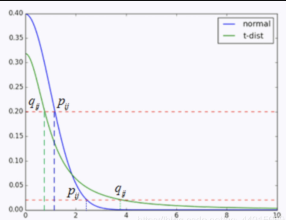
As shown in this figure, the x-axis represent the distant of two data points, the y-axis represents the probability \(p_{ij},q_{ij}\). If we replace the distribution of low-dimensional space with t-distribution, we will find that for two points that are close to each other, a shorter distance between them is required to maintain \(p_{ij}=q_{ij}\) compared to not using t-distribution, while for two points that are far away, a longer distance between them is required to maintain \(p_{ij}=q_{ij}\). This indicates that by replacing the distribution of low-dimensional space with t-distribution at the same level of KL divergence, similar points can be closer together and dissimilar points can be farther apart, which preserves the global characteristics of the original space. Thus, we can replace \(q_{i,j}\) with:

\[ q_{i,j} = \frac{(1+||y_j-y_i||^2)^{-1}}{\sum_{k\ne l}(1+||y_k-y_l||^2)^{-1}} \]

3.3 T-SNE

We then then obtained the procedures of the t- SNE algorithm:

1. Set the number of dimension to cut: \(X_{n \times m} \to Y_{n \times k}\). Randomize the initial value for \(Y\)
2. Set perplexity, usually among 5 ~ 50
3. For each point in X, calculate \(p_{i,j} = \frac{p_{j|i} + p_{i|j}}{2}\)
4. Calculate \(q_{i,j}\) for each point in Y. Calculate loss \(C\)
5. Update Y through momentum optimization
6. Repeat step 3~5, until the termination condition is reached

Although t-SNE partially alleviates the bias towards local information, overall t-SNE is still more suitable for visualizing local structures. Generally speaking, data with very high dimensions are not suitable for t-SNE. PCA algorithm can be used as a pre-step of t-SNE to maximize the retained variance and avoid overcrowding problems.

Comparing to PCA, which emphasize retaining as maximum variance(information) of feature, t-SNE focuses on retaining the similarity among data points, thus is more suitable for visualization rather than feature engineering. We can use t-SNE in combination with clustering algorithms to visualize the clustering results of high-dimensional data in two dimensions.

4. Linear Discriminant Analysis

4.1 Basic idea of LDA

Linear Discriminant Analysis (LDA) is another dimension reduction method that is commonly used for classification tasks. Given a labeled dataset, LDA finds a projection of the data that maximizes the separation between classes while minimizing the variance within each class.

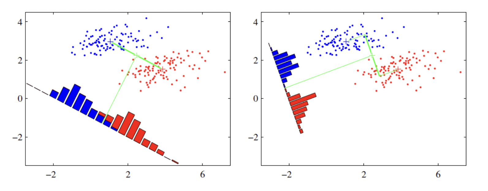
For example, in a dataset demonstrated as the figure, data point are labeled as red or blue. We want to map two-dimension data point into a one-dimension plane. According to the LDA, the plane in second plane is better, as the two cluster is dense and far away from each other.

Let the data set \(D = \{(x_1,y_1),(x_2,y_2),...(x_n,y_n)\}\), where each \(x_i\) is a m-dimension data points, \(y_i\) is its label \(y_i \in \{0,1...k\}\). Let \(\mu\) denote the mean vector of all sample, \(\mu_j\) denote the mean vector if all sample of category \(j\) . Assume the mapping we want LDA to conduct is \(Z = XP\)w, then the mapped mean vector \(\mu_y = \mu P\) . Let \(n_j\) denote the number of samples of category \(j\) , we define the variance between classes as:

\[ \begin{aligned} S_b' &= \sum_j (\mu_jP -\mu P)^T (\mu_ j P -\mu P) \\ & = P^T \sum_j (\mu_j-\mu)^T(\mu_j-\mu)P\\ & = P^TS_bP \end{aligned} \]

where \(S_b\) is the variance between classes of the original dataset. Samely we have the variance within classes:

\[ \begin{aligned} S_w' &= \sum_j^k S'_{w,j} \\ & = \sum_j^k \sum_{x\in X_j}(xP-\mu_jP)^T(xP-\mu_jP)\\ & = P^TS_wP \end{aligned} \]

where \(S_w\) is the variance with classes of the original dataset. Thus, we define the optimization function of the LDA as:

\[ J(P) = \frac{P^TS_bP}{P^TS_wP} \]

Since \(S_w,S_b\) are both matrix, we cannot apply function optimizer. Nevertheless, according to deduction in PCA, we know that ideally \(S_w'\) and \(S_b '\) should be diagonal matrix. We know for a diagonal matrix D we have \(|D| = \prod_i \lambda_i\) , where \(\lambda_i\) is the \(i ^{th }\) element on the diagonal. Suppose we want to reduct k dimensions to d dimensions, we can approximately change the optimization funtion to:

\[ J(P) = \frac{\prod_{diag}P^TS_bP}{\prod_{diag}P^TS_wP} = \prod_i^k\frac{P^TS_bP}{P^TS_wP} \approx \prod_i^d\frac{P^TS_bP}{P^TS_wP} \]

Based on the properties of the generalized Rayleigh quotient, we can derive that the maximum of \(\frac{P^TS_bP}{P^TS_wP}\) is the maximum eigenvalue of matrix \(S_w^{-1}S_ b\) , thus the maximum of \(\prod_i^d\frac{P^TS_bP}{P^TS_wP}\) is the product of the top d eigenvalue of \(S_w^{-1}S_ b\) , in this case, \(P\) consists of the eigenvectors of these eigenvalues. Notice that the maximum rank of \(S_b\) is \(k-1\), which decideds there are at most \(k- 1\) eigenvectors. This suggests that we cannot reduce the number of dimensions to more than \(k-1\) through LDA.

4.2 Procedures and Properties

Procedures

1. Given the dataset \(X_{n\times m}\) and label \(Y_{n \times 1}\), calculate \(S_w,S_ b\)
2. Calculate \(A = S_w^{-1}S_b\)
3. Conduct eigenvalue decomposition on \(S_w^{-1}S_b\) , select the top d eigenvalues and obtain matrix of according eigenvectors \(P'_{n \times d}\)
4. Calculate \(Z_{n\times d} = X P '\)

Properties

• Similar to PCA, LDA requires data to to be normally distributed
• The number of dimensions that LDA can reduct to is at most \(k-1\), where \(k\) is the number of category of \(Y\)
• When the information for classification are largely depends on the mean instead of the variance, LDA has better performance. On the contrary, when information are contained largely in variance, PCA has better performance.
• LDA can be used in classification. Since we project the original dataset into a low dimension space with label, we can obtain a distribution of low dimension points for each category of \(Y\). We can then apply parameter estimation to obtain a parameter \(\theta_j\) for each type \(j\) . When we have a new data point \(x\), we can map it into the low dimension space we found as \(z\) , calculate the probability of the mapped data points belonging to each category based on the estimated distribution parameters of each category:

\[ P(z \in Z _j ) = P_{\theta_j}(z) \]