K-Means and GMM

1. K-Means

1.1 About K-Means

K-Means is a typical unsupervised learning algorithm for clustering. It is a distance-based clustering algorithm.K-Means is a very interpretable algorithm.

We can understand K-Means from a EM algorithm perspective. The basic idea of K-means is to set a set of centers, and use the distance between a data point and all centers to decide which cluster the data point belongs.

Let a series of variable \(\mu = (\mu_1,\mu_2,...\mu_K)\) denote the locations of the centers.\(\mu\) represent a split plan of the clustering algorithm. For each data point \(x_n\), let \(r_n = (r_{n,1},r_{n,2},...r_{n,K})\) denote a group of variable indicating which cluster the data point belong to, where \(r_{n,k}\) is a binary variable(0 or 1). The objective of the K-means is to minimize the sum of distance between data points and center with a center: \[ J = \sum_n \sum_k r_{n,k} ||x_n-\mu_k||^2 \] This function is the objective function of a K-means algorithm, it is also called the distortion.

Using a EM algorithm:

• Initialization: Randomly Pick some data point
• Expectation: Given \(\mu\), optimize J about $r_n $ (find a best split)
• Maximization: Given \(r_n\), optimize J about \(\mu\) (update the center)

Training Process

Base on this idea, the training process of the K-Means is:

# Initialize Centers
centers = randomly select k data points as centers

# the terminate condition include:
#    E converge: The points in the clusters does not change(clusters_i+1 = clusters_i)
#    M converge: The location of centers does not change (mu_i+1 -mu < epsilon) 
while terminate condition is not reached
  # find a best split
  for each x in X:
      for each center in centers:
          dis_k = distance(x,center) #usually euclidean distance
          dis.append(dis_k)
      # the closet center is the cluster x belong
      x.cluster = minidx(dis)
  # update centers using the data points in to it
  for each cluster:
      cluster.center = cluster.x.mean()
		

Assumption & Properties:

1. The k must be a given number. This could be difficult in real application(K selection)
2. K-Means is a distance-based method, it require scaling of feature(Scaling)
3. K-Means is sensitive to the initial centers selection. Bad choice on initial centroids could trap the algorithm in local optimal. So K-Means could be unstable when the initial centroid change.(Initial centroid selection)
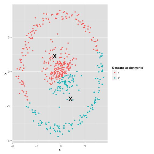
4. K- Means assume each cluster is a convex space(a sphere). Consider kernel functions when this assumption is not satisfied. (Kernel function)
5. K-Means assume a cluster is uniformly. This means K_Means can be unstable when there are outlier in the dataset or when some variable are not normally distributed. Consider outlier detection and normality transformation before using K-Means. (Normality)
6. K-Means assume the feature are not correlated. (Correlation Analysis)
7. K-Means require encoding on categorical variable, this could give binary variable very high variance, and overestimate the effect of them. (Categorical Variable Processing)
8. The traditional K-Means use euclidean distance, this assume different features(directions) have same importance(weights) to similarity. In real application, this assumption could not always been fulfilled. (Feature Weighting)
9. When a cluster actually exists in the space but fails to be recognized by the algorithm, we call it a hidden cluster. This can usually be caused by insufficient samples of that cluster(hidden clusters). K_Means cannot deal with imbalanced data hidden cluster.(Hierarchical Clustering)

Although K-Means has so many drawbacks, it still has wide application in industries. The core reason is that it is simple and interpretable, and there is only one hyper parameter to adjust. The unstable results is decided by the inner mechanism of K-Means. If we really cannot find a stable clustering results through K-Means, we should consider other algorithm.

2. Improvements on K-means

2.1 K-Selection

Score-K Plot(Elbow Method)

The Elbow method depict the relationship of the number of K and the performance of clustering. Let S denotes a metrics that can evaluate the performance of the clustering model. The elbow graph shows the S'value(on the y-axis) corresponding to the different values of K(on the x-axis). When we see an elbow shape in the graph, we pick the K-value where the elbow gets created. We can call this point the Elbow point. Beyond the Elbow point, increasing the value of ‘K’ does not lead to a significant reduction (or increase) in S.

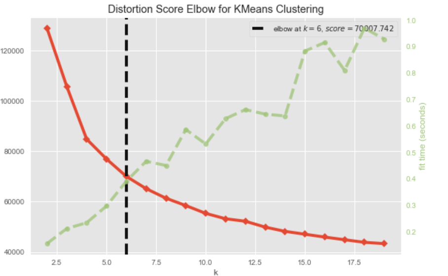
As shown in the picture, when K increase, the value of evaluating metric goes better while the cost of time being greater. Select the K with closest metrics value and time consuming as the elbow. The evaluating metric for the algorithm includes distortion, Silhouette Coefficient and Calinski Index. For details, refer to this article. Note that choosing K on a single metric can be verty biased, since some metrics prefer smaller K while other prefer greater K. Select the optimal K with multiple metrics taken into account.

ISODATA

The ISODATA is a improved kmenas model with embedded K selection method. Comparing to traditional Kmeans, it requires 4 parameter:

• \(K_0\): An expected number of K. The final K selection would be in \([{K_ 0 \over 2}, 2K_ 0]\)
• \(N_{min}\): the minimum number of data points in a cluster
• \(\sigma_{max}\): The max allowed \(\sigma\), where \(\sigma\) is a metric to measure the within distance in a cluster
• \(d_{min}\): The min allowed d, where d is a metric to measure the distance between two clusters

The training Process of the ISODATA is given as follows:

Initialize Centers

while terminate condition is not reached
  find a best split based on distance
  
  
  for each cluster in the K_0 clusters:
  		if the number of points in the cluster < N_min:
  				drop the cluster and label or data points in it with the nearest cluster
  				K = K-1
  				
	update the centroids of all clusters

  if K < K_0 / 2:
  # spliter some clusters into 2 clusters
  		For each cluster:
  				# calulate the sigma on each dimension(feature), and select the maximum
  				s_max = max(sigma_x1,sigma_x2,...)
  				if s_max > sigma_max and n > 2*N_min:
  						execute a kmeans on this cluster with K=2 to split it into two cluster
  				else:
  						forward
  if K > 2K_0:
  # Calculate the distance between each pair of clusters:
  		D = distance_matrix(Clusters):
  		while any D(i,j) < d_min:
  				merge cluster i and cluster j into one cluster
  				#update the centroid of the new cluster
  				c_temp = 1/(ni+nj)(ni*ci+nj*cj)
  				update D
  		
  # update centers using the data points in to it
  for each cluster:
      cluster.center = cluster.x.mean()

Such a algorithm can adjust the number of K in the dynamic training process.

2.2 K-Means++

The K-Means++ is an improved version of K-Means aimed at optimizing the initial centroids selection. Basically, it believe the more separated the initial centroids are, the more stable the clustering results will be. For the initial centroids choosing:

# randomly pick a data point
c1 = random(dataset)
centers.append(c1)

while len(centers) < k:
		for each sample s:
        # calculate the minimum of the distance between 
        D_s = min(dis(s, c1), dis(s,c2),....)
        D_s = D_s ** 2
        D.append(D_s)
     # Use the ratio of D[s] and sum of D as a probability of s being selected as a centroids
     Prob = D[s] / sum(D[s]) for s in all sample
		# decide the next centroid using a Roulette method
		r = rand(0,1)
		if  Prob[s-1] < r < Prob[s]:
			 # select s as a centroid
			 centers.append(s)

2.3 Kernel K-Means

Kernel K-means is an unsupervised clustering algorithm that extends the traditional K-means algorithm by incorporating the kernel trick. The kernel trick allows for clustering of non-linearly separable data by implicitly mapping the data points to a higher-dimensional feature space. By using kernel functions, we can compute similarity between data points in the higher-dimensional space without explicitly calculating their high-dimensional representations.

The specific difference is, when calculating the distance between two data points, we know use a kernel distance(kernel trick) to evaluate the similarity of 2 data point in a high dimension.

Choose a kernel function: Select an appropriate kernel function, such as the Gaussian Radial Basis Function (RBF), polynomial kernel, or Sigmoid kernel. The kernel function is used to compute similarities between data points in the higher-dimensional space.

For details of kernel function, refer to ongoing

2.4 K-Medoids

We can conduct outlier detection to elimate their influences. However, some points that are on the boundary of clusters would "pull away" the centroid we found. Consider a cluster \((1,2),(2,1),(1,1),(5,10)\), the last point would distinctly move the centroid in updating.

To fix such problems, we can introduce K-Medoids, which apply different centroid updating strategy. In K-Medoids, the new centroid is not the mean of all data points in the cluster, Instead, for each point \(x\) in the cluster, we need to compute the Manhattan Distance between \(x\) and every other data point. The sum of these distances is the error of point \(x\) : \[ \begin{aligned} Error(x_i) &= \sum_{j \ne i } ManhattanD(x_i,x_j)\\ centroid &= argmin_{x_i} \ Error(x_i) \end{aligned} \]

# Initialize Centers
centers = randomly select k data points as centers

while terminate condition is not reached
  # find a best split
  for each x in X:
      for each center in centers:
          dis_k = distance(x,center) #usually euclidean distance
          dis.append(dis_k)
      # the closet center is the cluster x belong
      x.cluster = minidx(dis)
  # update centers using the data points in to it
  for each cluster_k:
      for each x_i in cluster:
      		#calculate the sum of mahatten distance between point x_i and the rest point
      		for each x_j in rest points in the cluster:
      				error_ij = Mah_Dist(x_i,x_j)
      		error_i = sum(error_ij)
      		Error.append(error_i)
      # update the cent 
      center_k = argmin_x(Error)

Although K-Medoids can undermine the effect of points on boundary, the time complexity of updating centroids is \(O(n^2)\), which makes the whole algorithm time-consuming.

2.5 K-Means on Categorical Variable

K-means algorithm has issues when dealing with categorical variables. This is mainly because K-means relies on Euclidean distance to compute similarity between data points, which is meaningful for continuous variables but not applicable to categorical variables. Categorical variables are typically non-numeric data that cannot be directly used to calculate Euclidean distances. Even if you transform categorical variables into numeric values through some feature engineering method(such as one-hot encoding), it still doesn't capture their actual relationships.

To address this issue, we can adopt the following approaches to improve the K-means algorithm for handling categorical variables:

Alternative distance metrics:

For categorical data, you can use other distance metrics such as Hamming distance or Jaccard similarity. These metrics can better capture the relationships between categorical variables. When implementing K-means, you can replace Euclidean distance with one of these metrics. For details of Distance, refer to this article

An implementation of this method is the K-Modes algorithm. K-Modes is a clustering algorithm specifically designed for categorical variables. It works by replacing the Euclidean distance with the hamming distance and updating the cluster centroids using the mode instead of the mean. The matching distance is the number of mismatching attributes between two data points, for example a data point X = [1,2,5,3,0], and the centroid C = [1,2,4,2,3], then \(d_{match} = 3\)

K-Prototypes algorithm:

K-Prototypes is a hybrid of K-means and K-Modes algorithms. It is suitable for datasets containing both continuous and categorical variables. The K-Prototypes algorithm calculates a mixed distance based on the attribute type, combining the Euclidean distance for continuous variables with the matching distance for categorical variables. Similarly, updating the cluster centroids also requires considering both continuous and categorical variables separately.

2.5 Weighted K-Means

In the original K-Means algorithm, we eliminated the dimensional differences of each feature through scaling, and at this point, the importance of each feature for similarity calculation is equal. However, in real applications, this may not be true. If a feature contains very little information and a lot of noise, but has the same importance as other dimensions in distance calculation, then this feature will reduce the accuracy of clustering. Therefore, an improved algorithm, Weighted K-Means, was proposed to solve this problem. In WKMeans, we assign a weight to each feature, and the optimization objective function of clustering becomes: \[ J(C) = J = \sum_n \sum_k r_{n,k}\sum_i w_i^\beta(x_{n,i}-\mu_{k,i})^2 \] where \(\omega_i\) is the weight of the \(i^{th}\) dimension, \(\sum_i\omega_i = 1\). \(\beta\) is a parameter controls the extent of weighting, usually among \([0,1]\). When \(\beta = 0\), the WKMeans degenerated to the original K-Means algorithm.

In training procedures of the WK-Means, we need to update the weight vector after we update the centroids of all clusters in each iteration. With the Lagrange multiplier method, we can obtain the updating equation of \(\omega_i\) : \[ \omega_i = \frac{1}{\sum_j\frac{D_i}{D_j}^{\frac{1}{\beta-1}}} \] where \(D_j\) is the sum of unweighted distance of all samples to their corresponding centroid on the \(j^{th}\) dimension, \(D_j = \sum_n\sum_kr_{n,k}(x_{n,j}-\mu_{k,j})^2\).

2.6 Hierarchical Clustering

Hierarchical clustering is a type of clustering algorithm that aims to build a hierarchy of clusters. It can be classified in Agglomerative Clustering and Divisive Clustering.

The Agglomerative Clustering starts by considering all data points as individual clusters and then repeatedly merges the two closest clusters until there is only one cluster left, while in divisive clustering, the algorithm starts with all the data points in a single cluster and recursively splits them into smaller and smaller clusters, until the minimum number of samples in a cluster is reached.

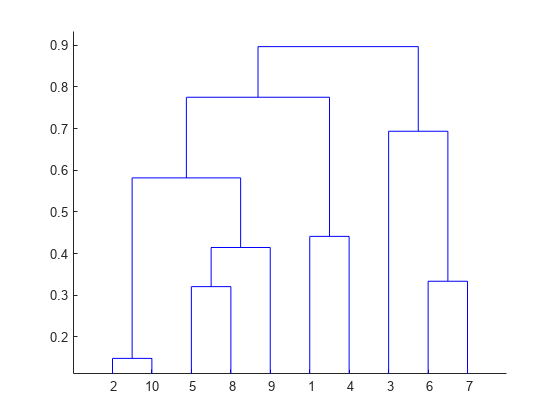
The result is a tree-like structure, called a dendrogram, that shows the hierarchical relationships among the data points.

img

The Divisive Clustering is easy to implement, we can simply repeat K-Means recursively on each hierarchy. The Agglomerative Clustering involves computing the similarly of two clusters when merging them, there are three metrics:

• Single Linkage: the distance between the two closest data points in the two clusters

img

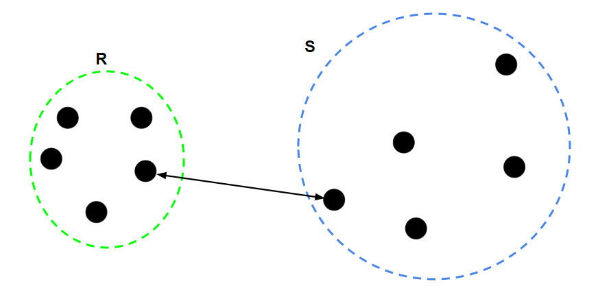
• Complete Linkage: the distance between the two farthest data points in the two clusters

img

• Compute the distance between each pair of data points in the two clusters。Calculate the mean of all distances as the distance between two clusters.

img

3. Gaussian Mixture Model

3.1 Mixture Model

A mixture model is a statistical model that represents the presence of subpopulations within an overall population, without requiring that an observed data set should identify the sub-population to which an individual observation belongs.

If we believe the distribution of each sub-population is a Gaussian distribution, then we call the whole model a gaussian mixture model: \[ P(x) = \sum_i^k \alpha_kN(x|\mu_k,\sigma_k) \] where \(\sum_ i^ k \alpha_ k = 1\), representing a weight that allows \(\int P(X = x) = 1\). In a clustering problem, we can use the probability that a random data point will belong to cluster k as the weight \(\alpha_k = P(z=C_k)\), in other word, the distribution of the hidden variable z, denoted as \(P(z) = (\pi_1,\pi_2,...\pi_k)\). Since we usually have multiple feature in clustering, the gaussian distribution is usually a mutilvariate normal distribution, replace \(\mu_k,\sigma_k\) with matrix of mean and covariance \(M, \Sigma\): \[ P(x) = \sum_i^{k}P(x|z=C_i)P(z=C_i) = \sum_i^{k}P(x|M_k,\Sigma ^2_k)\pi_k \] Thus, we find that the GMM model transform the clustering to a parameter estimating problem on \((M_1,...M_k),(\Sigma_1,...\Sigma_k),(\pi_1,...\pi_k)\).

3.2 EM Algorithm to Solve GMM

We can applied the EM algorithm to optimize the estimation of the three groups of parameters.

We know from the EM algorithm that for each point \(x_i\), the lower boundary of the likelihood function is: \[ Q_i(z_j) = P(z_j|x_i,\theta_j)=\frac{P(z_j)P(x_i|z_j,\theta_j)}{\sum_jP(z_j)P(x_i|z_j,\theta_j)}= \frac{\pi_jN(x_i|M_j,\Sigma_j)}{\sum_j^k\pi_jN(x_i|M_j,\Sigma_j)} \] The Likelihood function would be: \[ \begin{aligned} L(M,\Sigma,\pi) &= \sum_i^n\sum_j Q_i(z_j)log(P(x_i,Z_i = z_j|\theta_{j}))\\ & =\sum_i\sum_j \frac{\pi_jN(x_i|M_j,\Sigma_j)}{\sum_j^k\pi_jN(x_i|M_j,\Sigma_j)}log[\pi_jN(x_i|M_j,\Sigma_j)] \end{aligned} \] Through deriving, we can find the update equation for the parameters. Let \(\mu^{(t)}_{j}\) denote the estimation for mean of the \(j^{th}\) cluster in the \(t^{th}\) iteration: \[ \begin{aligned} M_{j}^{(t+1)} &= \frac{\sum_i^nQ_i(z_j) x_i}{\sum_iQ_i(z_j)}\\ \Sigma_j^{(t+1)} &= \frac{\sum_i^n (x_i - M_j^{(t+1)})^T\cdot (x_i - M_j^{(t+1)})Q_i(z_j)}{\sum_i^nQ_i(z_j)}\\ \pi^{(t+1)}_j &= \frac{\sum_i^nQ_i(z_j)}{n} \end{aligned} \] Thus the traning algorithm for GMM is:

1. Randomly initial \(M,\Sigma,\pi\)
2. For each sample, compute posterior probability \(Q_i(z_j)\)
3. Update \(M,\Sigma,\pi\) through the equations above
4. Repeat step 2-3, until termination condition is reached

3.3 About GMM

1. GMM is a probability model, the prediction yields the probabilities a data points belongs to each cluster
2. To predict a data point, fix \(M, \Sigma\), compute the probability it belongs to each cluster
3. Unlike K-Means, GMM is soft-clustering, K-Means can be saw as a hard clustering variant of GMM.
4. GMM directly model on \(P(X, Z)\), thus it is a generative model.

​