Expectation Maximization Algorithm(EM)

1. Baisc Idea of Expectation Maximization Algorithm

The Expectation Maximization Algorithm(EM) is a type of algorithm sharing the same basic idea. It's not a specific model but a way to solve problems like parameter estimation and clustering.

First, recall the formula of the Maximum Likelihood Estimation. Given a sample set, we suppose the variable follows a distribution \(P(X|\theta)\). According to MLE, we can estimate the parameter \(\theta\) by: \[ \theta = argmax \ \ ln[\prod_n P(X_n = x|\theta)] = argmax \ \ \sum_n ln[P(X_n = x|\theta)] \] Suppose we now have a hidden variable \(Z\) that has j possible values. We cannot directly read Z from the dataset. Under each possible value \(z_i\), X follows a unique distribution \(X \sim D(\theta = \theta_i)\). The Likelihood estimation function should now be: \[ (\theta, Z) =argmax \ \ \sum_n ln[\sum_i P(X_n = x,Z_n = z_i)|\theta_i)] \] For example, suppose we want to estimate the average height of a group of student. As we all known, the average height of male and female are different. \(H_m \sim N(\mu_1,\sigma^2_1),H_f \sim N(\mu_2,\sigma^2_2)\). Suppose we do not have the variable sex in our data set, but we do know there are two distribution, and we want to estimate both of them. In this case, when given a sample, there are actually two thing to do:

1. What's the gender(hidden variabl) of a sample?
2. Given the gender, update according distribution's average height(parameter)

We can see when we need a EM algorithm: There exists multiple distributions. We don't know which distribution a sample is drawn from, but we do know this process is decided by a hidden variable not collected in the data.

Now back to the equation of above, we know that finding out the derivatives of this function is difficult, as the log of the margin distribution \(log(\sum_z P( x, z))\)'s derivative is very hard to solve. In this context, we can transform the format: \[ \sum_n ln[\sum_i P(X_n = x,Z_n = z_i)|\theta_i)] = \sum_n ln[\sum_i Q(z_i)\frac{P(x,z_i|\theta_i)}{Q(z_i)}] \] Where we demand \(Q(z)\) is a new distribution such that: \(\sum Q(z_i)\)

according to the Jensen inequality, \(log(\sum_i\lambda_iy_i) \ge \sum_i\lambda_i[log(y_i)]\) , the equality is satisfied when \(y_i = c\).

Thus: \[ \iota(\theta,z|X) = \sum_n ln[\sum_i Q(z_i)\frac{P(x,z_i|\theta_i)}{Q(z_i)}] \ge \sum_n\sum_iQ(z_i)log\frac{P(x,z_i|\theta_i)}{Q(z_i)} \] According the condition of the equality fulfillment of Jensen inequality: \[ \begin{aligned} \frac{P(x,z_i|\theta_i)}{Q(z_i)} &= c \\ P(x,z_i|\theta_i)&= c Q(z_i)\\ \sum_i P(x,z_i|\theta_i)&= c \sum_i Q(z_i) = c\\ Q(z_i) &= \frac{P(x,z_i|\theta)}{c} = \frac{P(x,z_i|\theta_i)}{\sum_iP(x,z_i|\theta_i)}\\ &= \frac{P(x,z_i|\theta_i)}{P(x,|\theta_i)} = P(z_i|x,\theta_i)\\ \end{aligned} \] We now know that when we select \(Q(z_i) = P(z_i|x,\theta_i)\), what we get is a low boundary of the log likelihood function. We know that: \[ P(z_i|x,\theta_i) = \frac{P(z_i,x|\theta_i)}{P(x|\theta_i)} = \frac{P(z_i,x|\theta_i)}{\sum_iP(z_i,x|\theta_i)} \] Suppose the value of the hidden variable is \(z_i\), and the parameter of the distribution when \(Z = z_i\) is \(\theta_i\), the basic assumption of the problem can be solved by EM is, when \(\theta_i\) is fixed for a value, and the sample results x are given, we should be able to calculate the specific value of \(P(z_i,x|\theta = \theta_i)\)

Such a fact means, we can directly calculate \(Q(Z)\) from the observation on data. This save us from calculating the \(Z^*\) by \(\frac{\partial L}{\partial Z} = 0\), where \(Z^*\) denotes the optimal value of \(Z\) about L when \(\theta_i\) is fixed.

According to such assumption, the EM algorithm can be conclude as:

1. Randomly select a value for each \(\theta_i\) in the first iteration, denoted as \(\theta_{i,0}\)

2. Expectation: For each sample \(x_n\), calculate the posterior probability \(Q_n(z_i) = P(Z_n = z_i,X_n = x_n|\theta_i = \theta_{i,0})\). This step should yield a constant \(Q_n(z_i)\) for each \(z_i\) for each sample n.

3. Maximization: bring \(Q(z)\) back the likelihood function, since \(Q(z_i)\) is now a constant and do not have an influence to derivative, we can reformat the likelihood function as: \[ \theta_{i,1} = argmax \ \ \sum_n\sum_i Q_n(z_i)log(P(x_n,Z_n = z_i|\theta_{i,0})) \]

4. Let \(\theta_i = \theta_{i,1}\), repeat step 2-4, until \(\theta\) converge

2. Example of EM

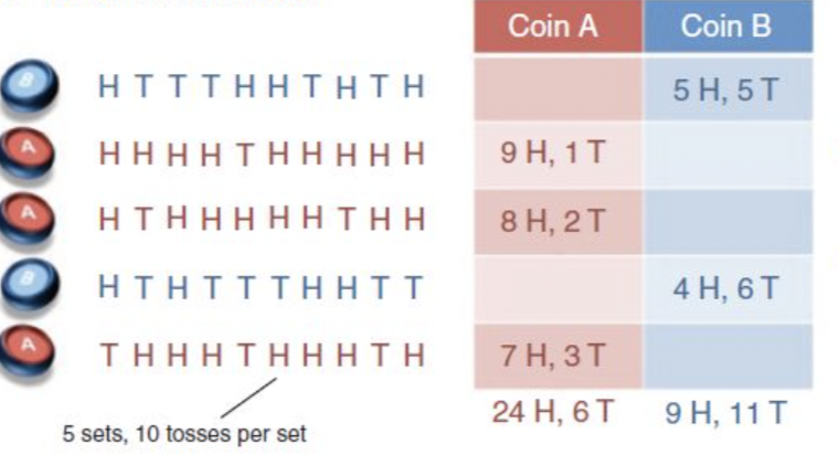
Suppose we have 2 coin A and B, each with a different probability \(p_1,p_2\) of flipped as a head. We randomly select a coin and flip it 10 times and call it a trail. We repeat 5 trail and obtian 5 samples. Let:

• \(X_n\) denote the number of heads in the \(n^{th}\) trail
• \(Z_n\) denote the selection of coin in the \(n^{th}\) trail
• \(\theta_{A,k}, \theta_ {B,k}\) denote the estimation of \(p_1,p_2\) in the \(k^{th}\) iteration

suppose we have the following data(unlike shown in the picture, we do not know which coin is selected). Suppose the prior knowledge \(P(Z =A) = \frac{1}{2}\) is fixed, and we do not want to update it.

Step 1

Initialize \(\theta_A = 0.6, \ \theta_ B = 0.5\)

Step 2

when \(Z = A, \theta = \theta_A\), now looking are the data of the first trail \[ \begin{aligned} P(Z_1 = A|X_1,\theta_{A,1}) &= \frac{\frac{1}{2} P(Z_1 = A, X_1=5|\theta_{A,1} = 0.6)}{\frac{1}{2}P(Z_1 = A, X_1=5|\theta_{A,1} = 0.6) + \frac{1}{2}P(Z_1 = B, X_1=5|\theta_{B,1} = 0.5)} \\ & =\frac{0.6^5*(1-0.6)^5}{0.6^5*(1-0.6)^5 + 0.5^5*(1-0.5)^5} \\ & = 0.45 \end{aligned} \]

Samely, \(P(Z_1 = B|X_1,\theta_{B,1})\) is 0.55. Repeat the calculation for each of the \(n\) trails. Let the last posterior probability be \(\mu_{A, n} = P(Z_n = A|X_n,\theta_{A,1}), \quad \mu_{B, n} = P(Z_n = B|X_n,\theta_{B,1})\)

Step 3

Format the likelihood function: \[ \begin{aligned} L(\theta_{A,1},\theta_{B,1}) &= \sum_n \sum_{z_i}P(Z_n = z_i|X_n,\theta_{z_i,1})\ logP(X_n, Z_n|\theta_{z_i,1})\\ & =\sum_{n=1}^5 \mu_{A,n} log(\theta_{A,1}^{X_n}(1-\theta_{A,1})^{10-X_n} ) + \mu_{B,n}log(\theta_{B,1}^{X_n}(1-\theta_{B,1})^{10-X_n} ) \end{aligned} \] Step 4

Now find the partial derivatives of the Likelihood function and let them euqals to 0, updated the parameters by the optimal value. \[ \theta_{A, 2} = \theta_{A,1}^* = solve (\frac{\partial L_1 }{\partial \theta_{A,1}} = 0) \]

\[ \theta_{B, 2} = \theta_{B,1}^* = solve (\frac{\partial L_1 }{\partial \theta_{B,1}} = 0) \]

3. Application of EM Algorithm

The application of the thought of EM algorithm includes:

• K-Means and GMM
• Sequential Minimal Optimization in SVM
• HMM