Decision Tree and Ensemble Models

1. Decision Tree

1.1 About Decision Tree

Decision Tree is a data structure that can split data into subsets. In Machine Learning, we can use such a structure as our hypothesis space to segment our datasets into units and perform prediction.

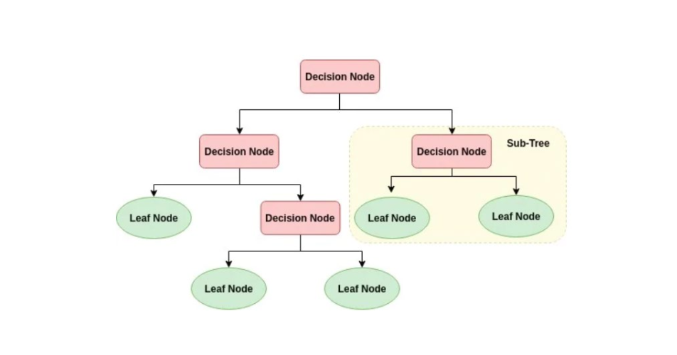
A decision tree consists of decision nodes and leaf nodes. Each decision node represent a split of sample based on some conditions a input feature \(X_i\). A directed route of the decision nodes represent a series of conditioning on the sample sapce. Each leaf node represents a subsample space obtained from a unique route, and we can estimate the conditional probability distribution \(P(Y|X=x)\) from the leaf node. The output variable Y can be either continuous(regression) or discrete(classification).

The decision tree is a non-parameter model. It can be infinitely extended without a constraint on max tree depth.

1.2 Training Process

The training process of decision tree is a recursive process. Let D denote the original sample set, X denote the feature spaces

def splitting(tree):
		while impurity metrics is not reached:
				x+i = select a feature x_i in feature space X(tree)
				sub_tree_left,sub_tree_right = find the best split based on x_i(tree, x_i)
				tree.left = splitting(sub_tree_left)
				tree.right = splitting(sub_tree_right)
	  return tree

splitting(D)

def label_and_predict(tree, sample):
		for leaf in tree:
				if a classification_tree:
						# use the mode of Y of training samples belong to this leaf node as the prediction
						leaf.pred = leaf.Y.mode()
				else:
						# use the mean of Y of training samples belong to this leaf node as the prediction
						leaf.pred = leaf.Y.mean()
	
		leaf_node_for_sample = find the leaf node the sample belong to according to sample's X
		sample_pred = leaf_node.pred

The implementation of Decision Tree includes ID3, C4.5 and CART. The differences of these implementations are the strategy they select layer(feature) and best split.

2. Implementation of Decision Tree

2.1 ID3

ID3 is a decision tree that can deal only with finite discrete inputs(usually categorical features). Suppose we have a sample set D and a feature space X, where \(X_i\) is a finite discrete feature like sex, country. If \(X_i\) has infinite values or is continues, then the ID3 requires the feature to be binned into finite discrete sections.

2.1.1 Feature Selection and Splitting

The strategy of selecting feature to split is based on Information Gain. For the explanation of IG, refer to this article.

For each feature \(X_i\): \[ \begin{aligned} IG(X_i) &= H(D) - H(D|X_i) \\ &= -\sum_m^k p(y=c_m)log(p(y=c_m)) - (-\sum_n\sum_m p(y=c_m|X_i = x_n)p(X=x_n)log(p(y=c_m|X_i = x_n))) \end{aligned} \] According to the definition, the feature with the largest imformation can reduce the uncertainty of Y to the greatest extent, thus would be selected as the feature to split. There is no specific techniques in finding best split, since all features are categorical, just split the tree into n nodes, where n is the number of categories of feature \(X_i\)

2.1.2 Properties

• ID3 does not have any pruning strategy
• ID3 perfer features with large number of category
• ID3 can only deal with finite discrete inputs if no binning is implemented.
• ID3 cannot deal with missing values
• Since or feature is catrgorical, once a featrure is selected a layer, it would not appear in the following subtrees any more.

2.2 C4.5

C4.5 is a improved version of ID3. One drawback of ID3 is that it would perfer features with large number of category. For example, if there is a unique identity number for each sample, then that feature's IG would be 1, but this provide no clues for future's prediction.

2.2.1 Feature selection and splitting

To solve this, the C4.5 use Information Gain Rate to select feature: \[ IGR(X_i) = \frac{IG(X_i)}{H(D)} \] this would penalize those features with to many categories, as these features usually have larger entropy. However, this could bring the algorithm to the opposite that it would prefer feature with less number of categories. This means the absolute values of IG can be low while the IGR is high. To fix this, the C4.5 would first do a feature selection based on IG:

for X_i in X:
		if IG(X_i) < IG(X).avg()
		X.drop(X_i)

In addition, the C4.5 introduce different techniques to deal with selection on continuous input feature, for a continuous feature \(X_i\):

for X_i in X
		if X_i is continuous:
      Sort all sample by X_i in a ascending order
      for each adjacent samples
          m_j = the medium of X_i_j,X_i_(j+1) #use the medium as a threshold
          #Z is a label flagged whether X_i of a sample is above the threshold
          Z = Z_right if x_i_j < m_j else Z_right 
          IGR_j = IGR(D, Z) #A binary split based on Z
      # The split with the highest IGR is the best split of feature X_i
      IGR_best_i = max(IGR_j)
    else:
    		IGR_best_i = calculate IGR(X_i) as a categorical variable like ID3
    
# Compare all
the feature to select = argmax_Xi(IGR_best_i)
		

The process put feature selection and feature splitting together. It first use a enlightening method to filter some feature with low IG. then calculate the IGR for the rest of the features. For a continuous feature, it use the split with highest IGR as the best split. For a categorical feature, it still generate a child node for each category.

2.2.2 Pruning Strategy

One drawback ID3 is that it does not have a pruning strategy, thus can be easy to overfit. In C4.5, post-pruning is applied to control the complexity of the model. The post-pruning means the algorithm would first make the split and then decide whether to prune the subtrees based on the error rate on the leaf node. Specifically, the post-pruning strategy is a method called Pessimistic Error Pruning.

For a decision node, suppose the algorithm first split \(n_L\) child nodes based on a feature. Then:

• Let \(E_i\) denote the number of false classification in the \(i^{th}\) node
• Let \(N_i\) denote the number of samples in the \(i^{th}\) node
• Let \(\gamma\) be a penalty parameters for complexity of model

The error rate of splitting and treat the node as a subtree: \[ e_{tree} = \frac{ \sum_iE_i + \gamma*n_L}{\sum_iN_i} \] Consider a random variable \(M_{tree}\) denoting the number of misclassification. For example, if the output variable Y is binary, we can consider \(M_{tree} \sim Bino(e,\sum_i N_i)\) $$ \[\begin{aligned} E[M_{tree}] &= \sum_iN_i *e_{tree}\\ Std[M_{tree}] &= \sqrt{\sum_i N_i*e_{tree}*(1-e_{tree})} \end{aligned}\]

\[ Now apply pruning and replace the subtree with a leaf node. Let E, N denote the number of misclassified samples and all samples in the leaf node, calculate the error rate if not splitting and treat the node as a leaf node: \] e_{leaf} = \[ Accordingly: \] E[M_{leaf}] = N*e_{leaf} \[ If $M_{leaf}$ is significant greater than $M_{tree}$, we can make the judgement that the splitting is necessary. When N is big, the binomial distribution is approximate to a Normal distribution. Thus, through a test,the condition of accepting a splitting is: \] p = T_test(E[M_{leaf}] - E[M_{tree}]) $$ Otherwise, the subtree should be pruned.

2.2.3 Missing Value Processing

When there exists missing values in features, two problem needs to be solved by the decision tree:

• How to calculate the IG/IGR of \(X_i\) when there are missing values in \(X_i\)?
• When training, how to decide which sub-node the sample containing missing value belong?
• When predicting, how to label the sample when it meet a node that based on its missing values?

For the first question, the solution by C4.5 is to calculate the IGR on samples without missing values and then add a weight to the IGR. Let the weight be: \[ \rho = \frac{n_{\widetilde{D}}}{n_D} \] where \(D, \widetilde{D}\) is the orginal sample set and a subset that samples with missing values of \(X_i\) are dropped. \(n\) denote the number of samples. The revised IGR would then be: \[ IGR(X_i)'/IG(X_i)' = \rho * IGR(X_i)/IG(X_i) \]

For the second question, let \(w_k\) denote the fraction of samples that belong to the \(k^{th}\) category(or value for continuous variable): \[ \omega_k = \frac{n_k}{n_ {\widetilde{D}}} \] If a sample's value on \(X_i\) is missing when trying to split the samples based on \(X_i\), then those missing value samples would enter every child node with a weight \(\omega_k\). This means, when further splitting the nodes, the \(P(y = c_m)\) in the information gain now calculated as: \[ P(y = c_m) = \frac{\sum \omega_{k, y= c_m}}{\sum \omega_k} \] and the weight of information gain would also be: \[ \rho = \frac{\sum\omega_\widetilde{D}}{\sum \omega_D} \] For example, suppose we have the following dataset

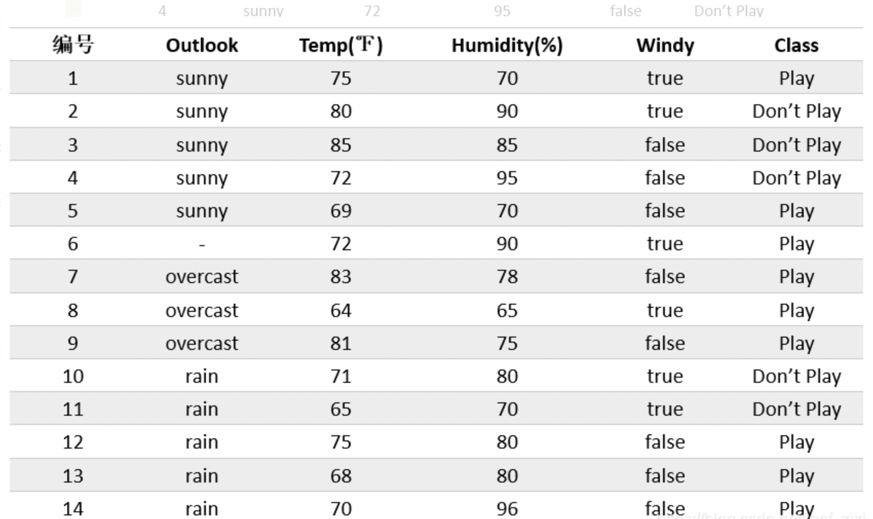
In this first split, \(\widetilde{D} = \{1,2,3,4,5,7,8,,9,10,11,12,13,14\}\), \(\rho = \frac{13}{14}\), then \[ \begin{aligned} H(\tilde{D}) &= [-\frac{5}{13}*log(\frac{5}{13})-\frac{3}{13}*log(\frac{3}{13})-\frac{5}{13}*log(\frac{5}{13})]\\ IGR &= \frac{H(\tilde{D}) - H(\tilde{D}|outlook)}{H(\tilde{D})}\\ IGR' &= \frac{13}{14}*IGR \end{aligned} \] Suppose outlook is the feature with max IGR'. Let split the sample based on outlook. Since there is a sample 6 that missing value "outlook", let will enter each node with a weight. \(\omega_s = \frac{5}{13}, \omega_o = \frac{3}{13}, \omega_r = \frac{5}{13}\)

Now move the subtree that "outlook = sunny"

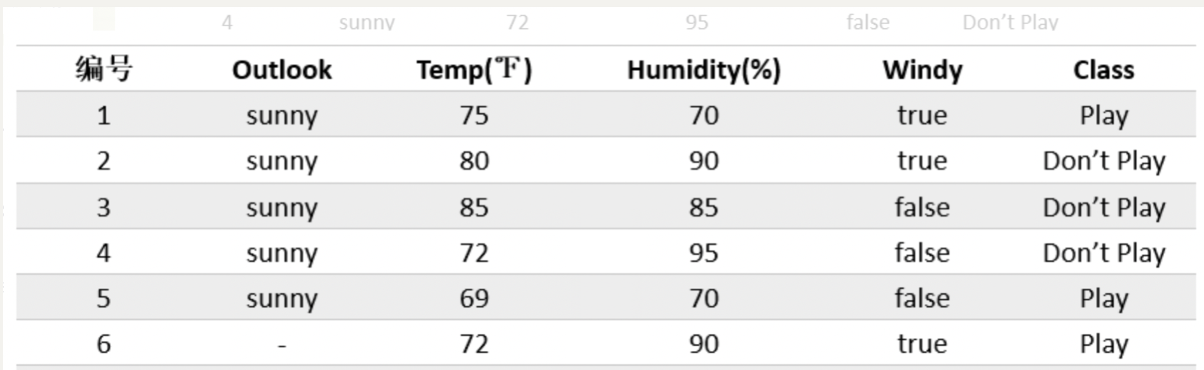
suppose we want to further split the tree and we want to calculate the IGR of "Windy", now: \[ \begin{aligned} \rho &= \frac{5+\frac{5}{13}}{5+\frac{5}{13}} = 1\\ H(\tilde{D_s}) &= [-\frac{2+\frac{5}{13}}{5+\frac{5}{13}}*log(\frac{2+\frac{5}{13}}{5+\frac{5}{13}})-\frac{3}{5+\frac{5}{13}}*log(\frac{3}{5+\frac{5}{13}})]\\ IGR &= \frac{H(\tilde{D_s}) - H(\tilde{D_s}|Windy)}{H(\tilde{D_s})}\\ IGR' &= 1*IGR \end{aligned} \]

Finally, for the third question, when we try to make the prediction. Suppose we have a decision tree like this:

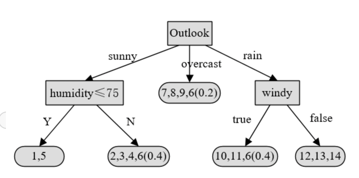
Now we have a sample that "outlook = sunny" and "humidity = null". To decide the label of this sample, we just calculate the conditional probability distribution of Y when the sample meet the node it is missing value of.

For the humidity node: \[ \begin{aligned} P(Class = play|sunny) =& P(Class = Play|Humidity \le 75|sunny) P(Humidity \le 75|sunny) \\ &+ P(Class = Play|Humidity > 75|sunny) P(Humidity > 75|sunny)\\ =&\frac{2}{5.4}*1+\frac{3.4}{5.4}*\frac{3}{3.4} = 44\% \end{aligned} \]

\(P(Class = Play) < P(Class = not \ play)\), thus the prediction is "play"

2.2.4 Properties

• C4.5 is a classification algorithm. Although it deal with continuous features, the output features still needs to be categorical
• For continuous feature, C4.5 sort the samples and split the samples into 2 parts. The continuous feature can be applied again in the subtrees.
• For categorical feature, C4.5 still split the samples into n parts. The categorical feature won't be applied again in the subtrees.
• C4.5 is still a Multi-tree. It has lower efficiency than CART.

2.3 Classification and Regression Tree(CART)

The C4.5 algorithm can only deal with classification tasks, and the efficiency of it is low. CART is a improved algorithm for C4.5.

2.3.1 Feature selection and splitting

CART has similar processing like C4.5, which sort the samples in an ascending order and find a best split to segment the samples in 2 parts. The difference is CART applies such method on all feature, not just continuous features, and it provides a different metrics to measure a split.

In addition, CART can do both regression and classification. When the output variable is continuous, it use a combined MSE to measure the error of a split: \[ MSE = [\sum_{i \in D_{left}}(y_i-\bar{y}) + \sum_{i \in D_{right}}(y_i-\bar{y})] \] When doing classification, CART use the Gini Index as a metric: \[ G = 1- \sum_i^mP(y = c_m) \]

\[ Combined \ Gini = G_{left} + G_{right} \]

Unlike information gain, both metrics are better when lower.

The feature selection process would then be:

for X_i in X
      Sort all sample by X_i in a ascending order
      for each adjacent samples
          m_j = the medium of X_i_j,X_i_(j+1) #use the medium as a threshold
          #Z is a label flagged whether X_i of a sample is above the threshold
          Z = Z_right if x_i_j < m_j else Z_right
          #A binary split based on Z
          if a regression tree:
          		I_j = combine_MSE(D, Z)
          else:
          		I_j = combined_Gini(D,Z)
      # The split with the lowest MSE or Gini is the best split of feature X_i
      I_best_i = min(I_j)

    
# Compare all
the feature to select = argmax_Xi(I_best_i)

2.3.2 Pruning Strategy

The pruning strategy applied in CART is called Cost Complexity Pruning. It is also a kind of post-pruning. The idea of this strategy is similar like Pessimistic Error Pruning in C4.5, but it works different.

Suppose we have a parent node t. Let \(T\)be tree below node t(\(T\) use t as a root node). Let C be error function that can evaluate the performance of \(T\). For regression, C can be MSE, for classification, C can be misclassification rate. Construct a regularization term \(C_\alpha\): \[ C_\alpha(T) = C(T) + \alpha|T| \] where |T| is the number of leaf nodes in T, \(\alpha\) is a hyperparameter that adjust the penalty of complexity.

Similarly like the C4.5, we calculate the difference on \(C_\alpha\) between use the tree T and replace T with a single leaf node. Define the cost of doing so as: \[ g(t) = \frac{C_\alpha(T_{leaf}) - C_\alpha(T_{tree})}{|T|-1} \] \(g(t)\) represent the cost on performance if replace the non-leaf node t with a leaf node.

The pruning strategy is then:

non-leaf nodes sorted = sort the non-leaf nodes in original DT from the bottom to the top
for node in non-leaf nodes sorted:
		# calculate the cost of each node
		cost_nodesa.append(g(node))
# fine the node with least cost and prune that node
node_to_prune = argmin(cost_node_i)
DT_temp = replace node_to_prune with a leaf node
# once a node is pruned, record the updated tree
DTs.append(DT.temp)

# validate each tree in the record and select the best
for DT_j in DTs:
	validate the performance of DT_j
select the DT_j with best performance

2.3.3 Missing Value Processing

Back to the three questions:

• How to calculate the MSE/Gini of \(X_i\) when there are missing values in \(X_i\)?
• When training, how to decide which sub-node the sample containing missing value belong?
• When predicting, how to label the sample when it meet a node that based on its missing values?

For the first question, the solution by CART is same as C4.5, which is give the MSE or Gini with a weight: \[ \rho = \frac{n_{\widetilde{D}}}{n_D} \]

where \(D,\tilde{D}\) is the orginal sample set and a subset that samples with missing values of \(X_i\) are dropped. n denote the number of samples.

The Gini/MSE would then be: \[ Gini'\ or \ MSE' = \frac{ 1}{\rho} * (Gini\ or \ MSE) \]

For the scond and third question, the CART use a method call surrogate splitter. Suppose we select \(X_i\) from X as our best splitting feature. If a sample reach the splitter with missing value on \(X_i\):

IG = Gini or MSE of the Decision node on X_i

thresh = a threshold measure the difference of IG on two feature

for X_j in the X except for X_i:
		IG_j = calculate Gini or MSE of X_j on current decision node
		# record X_j as a surrogate splitter
		SS.append(j, IG_j)
# rank the surrogate splitters according to there information gain

SS = SS.rank by S_j
for j,IG_j in enumerate(SS):
		if sample.X_j is missing: drop X_j from SS
		if IG - IG_j > thresh: drop X_j from SS
		if there are surrogate splitter left in SS:
				decide the sample based on X_SS[0] #decide the sample by the best surrogate splitter
		else:
				let the sample enter the leaf node with most samples in it
		

In this method, for a best spliter node \(X_i\), if a sample happen to miss value \(X_i\), we will calculate the MSE or Gini of the rest features based on the samples in this node. We rank these features by Gini or MSE and apply them as a surrogate splitter.

Given a sample, a legal surrogate splitter should guarante:

• The sample should not miss its value on the feature this splitter based on
• The surrogate splitter should not be too different too the original splitter, that is, the difference between there Gini or MSE should be within a threshold

In the legal surrogate splitters, select the best(with lowest Gini or MSE) surrogate splitter to decide which child node the sample should go to. If there are no legal surrogate splitters, just put the sample into the node that have the most samples.

This method is very time-consuming, as it demands metrics calculation on all features in every split.

2.3.4 Properties of CART

• CART can deal with both Regression and Classification
• Features in CART would be applied as splitters repeatedly. We can use the frequency they emerge as a feature importance measure
• CART is a strict binary tree, and it does not involve log calculations, thus is faster than C4.5
• CART has different pruning and missing value processing strategy comparing to C4.5
• CART suit big sample, the variance can be high if applied on small sample

3. Ensemble Model

As single model can have problem with bias or variance. An ideal is to combine multiple basic learner(single model) into a strong learner(ensemble model). The way to combine the basic learners includes:

Bagging

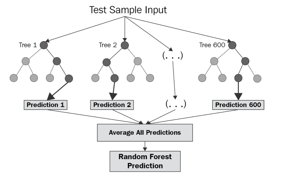
Bootstrap aggregating is a method to deal with high variance of model.It randomly take samples with replacement from the original dataset. Each subset is sent to a weak learner and used to estimate the probability \(P(Y|X)\). All weak learner work parallelly. When a new sample sent to the model for prediction, it would go through all weak learner and get a set of partial prediction. The weak learners would than make a vote to decide the final decision by the strong learner.

Boosting

Boosting is a method to deal with high bias of model. The bias is reflected by the residual between \(y_{true}\) and \(y_{pred}\). We can thus model on the residual again to get more accurate model. Boosting is a kind od serial method.

As a typical non-parameter learner, Decision is often applied as a basic learner in ensemble model.

3.1 Random Forest

3.1.1 Training Process

A random forest is a bagging method in which every learner is a decision tree. The basic learner is a CART, but in most applications, the basic learner support Information Gain as a splitting criterea when doing classification.

Specifically, the train process of a RF should be like:

1. Randomly take n sample set from the dataset with replacement, where n is the number of weak learner. Each sample set contain m samples
2. For each subset, conduct a column sampling, which take a subset k from the original feature space X
3. Train each weak learner with a sub training set with a size of \(m * k\).
4. For a test sample, run the test sample through each tree, then average each tree’s prediction.

3.1.2 Pruning Strategy

Since the bagging method already realize a overfitting control, usually we won't apply pruning on an RF. We can still demand pruning, if we do want so, based on the pruning strategy of a single DT though.

3.1.3 Missing Value Processing

Although weak learner already provides missing value processing strategy, it could be very time-consuming when applied to ensemble model with larger scale of estimators. Thus, most ensemble model frameworks do not provide missing value processing function in ensemble modeling.

However, if we do want to equip the RF model with a missing value imputation method, we can do the following stuff:

1. impute all numerical missing value with sample average, all categorical missing value with sample mode
2. use the imputed sample set to calculate a similarity matrix among all samples, where the similarity between the \(i^{th}\) and \(j^{th}\) samples is \(W_{i, j}\)
3. Back to the original sample set, use the similarity as a weight, fill a missing value \(X_{k,j}\), with the weighted average of all other sample: \(X_{k,j} = \frac{1}{n} \sum_{i\ne k}^n W_{i,k}X_{i,j}\). If \(X\) is a categorical variable, use a weighted vote.

This process is basically a data filling based on collaborative filtering

3.1.4 Feature Importance

Ensemble models usually have some embedded feature importance evaluation method. For the RF, there commonly are two methods:

Mean Impurity Decrease / Error Decrease/ Information Gain

For a feature \(X_i\), its importance on a non-leaf node m is: \[ FI(X_i,m) = GI_m -(GI_{left}+GI_{right}) \] Where GI is the gini index of the node, left and right represent the left and right child node of m.

Suppose in a DT, M is the collection of a node that select \(X_i\) as a spliter, then the feature importance of \(X_i\) on this tree is: \[ FI(X_i,DT) = \sum_{m \in M} FI(X_i,m) \] Suppose there are n trees in the forest, the feature importance of \(X_i\) would then be: \[ FI(X_i) = \sum_j^nFI(X_i,DT_j) \] We can normalize the feature importance so its scale is 1: \[ \hat{FI(X_i)} = \frac{FI(X_i)}{\sum_i FI(X_i)} \] Samely, we can replace the criterion with MSE or Imformation Gain and compute according feature importance

OOB Error(Permutation)

IN a RF, for a DT, there would exist some samples that never been selected by the bootstrap process. We call these samples the Out-of-bag data. We can use these data to evaluate the trained DT. Let \(E_j\) denote the error rate (1-accuracy) of the \(j^th\) DT using OOB data.

Now add a random noise to feaure \(X_i\), and use the OOB data with noise to evaluate the DT again. Denote the error as \(E_j'\)

If a noise added to \(X_i\) would lead to a great descent of accuracy of the DT, then \(X_i\) is very important to that DT. Thus we define the feature importance of \(X_i\) on the forest with n trees as: \[ FI(X_i) = \sum_j FI(X_i,DT_j) = \sum_j (E_j - E'_j) \]

3.2 Gradient Boosting Decision Tree(GBDT)

3.2.1 Training Process

In the GDBT, we define the residual as: \[ r = \frac{\partial L(y_{ture},M(X)) }{\partial M(X)} \] where L is a loss function, M(X) is the output of a tree

Let \(X_0,Y_0\) be the original inputs and outputs. According to the idea of boosting, the traning process of a GBDT is:

1. Fit a model \(M0\) to predict \(\hat{Y_0} = M_0(X)\)
2. Calculate the residual \(r_0 = \frac{\partial L(\hat{Y_0},Y_0)}{\partial\hat{Y_0}}\)
3. Fit a new model \(M1\) using X as inputs and \(r_0\) as outputs, get the prediction of residual \(\hat{r_0} = M_1(X )\)
4. update the prediction \(\hat{Y_1} = \hat{Y_0} + \alpha \hat{r_0}\), where \(\alpha\) is the learning rate
5. use \(\hat{Y_1}, Y_0\) to calculate \(r_1\), this time \(r_1 = \frac{\partial L(\hat{Y_1},Y_0)}{\partial\hat{r_0}}\)
6. Repeat process 3-5 until the residual is small enough

GDBT for Classification

GDBT requires the residual to be continuous, this means the basic learner of GBDT are all Regression Tree. But GBDT can still do classification. The idea is the same as Generalized Linear Model like Logistic Regression. For the weak learner to predict \(\hat{r_i}\), the weak learner first estimates a canonical parameter \(\theta\) for a Nature Exponential Family Distribution. Let \(\eta = M(X)\) denote the estimation of \(\theta\) given by the DT: \[ \hat{r_i} = AF(M_{i+1}(X)) = AF(\eta_{i+1}) \] where AF is the activation function. \[ \hat{Y_{i+1}} = \hat{Y_{i}}+\alpha\hat{r_i} = \hat{Y_{i}}+\alpha AF(\eta_{i+1}) \] Note thar the GDBT always \[ r_{i+1} = \frac{\partial L(\hat{Y_{i+1}},Y_0)}{\partial \eta_{i+1}} \] The loss function in classification scenarios are usually Log Loss.

For details of GLM, refer to this article

Subsampling

In many framework, GDBT support sampling. Suppose we have 100 feature and the subsampling rate is 0.9, the every time a new weak learner is created, 90 sample is drawed randomly from the sample set. This could lead to a situation that for model \(M_{i+1}\), the output variable for some samples are \(r_i\), while other samples's output is \(r_{j < i}\). Such a process would increase the bias but can reduce the variance of the model.

3.2.2 Pruning Strategy

Some GDBT support pre-pruning, that is, the impurity decrease or information gain must be less or greater than a threshold for the split the be generated. Samely, we can applied the post-pruning strategy the weak learner has originally.

However, in real application of boosting, we usually control overfitting by

• constrain the max depth of a single tree
• set a shrinkage parameter to \(\alpha\) to control the step size of learning
• Apply subsampling

3.2.3 Missing Value Processing

In GDBT, for time-saving reasons, the strategy is to:

1. When training, calculate impurity or information gain without missing value sample
2. Try to put all the missing value samples respectively into the left and right split and calculate which would bring less loss(based on the loss function selected). Put the sample into that split and record the direction(left or right)
3. When predicting, suppose a sample is missing value \(X_i\) and meet a node split on that feature. If there exists value missing on that node, then find the direction that missing values samples goes during the training process. If there are no missing value samples in the training, then the new sample goes to a default direction decided by the instance.

3.2.4 Feature Importance

The GDBT can use same feature importance evaluation method like the RF. Since GDBT's basic estimator is Regression Tree, we usually just calculate the decrease of MSE. However, when doing classification, we can also consider directly use the real label Y to calculate the impurtiy of a node.

3.3 XGBoosting

3.3.1 Training Process

Objective Function

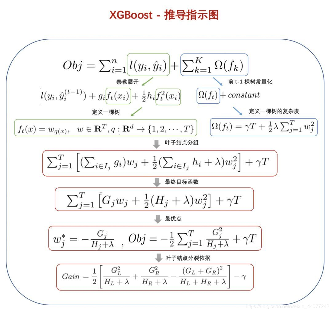
The XGboosting is a improved version of GDBT. The biggest difference is the way it define the residual. XGB use the second derivative Taylor Series to define the residual, that: \[ \begin{aligned} r_{i+ 1} &= [L(y_0,\hat{y}_{i})+g_{i}\hat{r}_i+\frac{1}{2}h_{i}\hat{r}_i^2] + \Omega(T)\\ g_{i} &= -\frac{\partial L(y_0,\hat{y}_{i})}{\partial M_{i+1}(X)} \\ h_{i} &= -\frac{\partial^2 L(y_0,\hat{y}_{i})}{\partial M_{i+1}(X)^2 } \\ \end{aligned} \] where in regression \(\hat{r_i} = M_{i+1}(X)\) and in classification \(\eta_ {i+ 1} = M_ {i+1}(X)\), and \(\Omega(T)\) is a regularization term: \[ \Omega(T) = \gamma J + \frac{1}{2}\lambda \sum_{j=1}^J b_j^2 \] where J is number of leaf nodes under node T, \(b_j\) is values on those leaf nodes, \(\gamma, \lambda\) are hyper parameters control the degree of penalty.

Splitting Strategy

Unlike traditional CART, the XGB use a generalized gain deduced from the objective function.

Let \(R_ j\) represent the collection of samples belong to the current node t. In equation 32, we know that the prediction of residual on a node t \(\hat{ r}_t\) is actually decided by the samples, which is the average of samples beneath the t's subtree, which is the leaf values \(b_j\). If we express \(r_i\) in \(\sum_j^ Jbj\): \[ r_t = [L(y_0,\hat{y}_{i})+G_{j}b_j+\frac{1}{2}(H_{j}+\lambda )b_j^2] + \gamma J \] where \(G_j = \sum_{k \in R_j}g_k\), representing the sum of first derivatives of samples belong to this node. Same with \(H_j\).

When the samples belongs to the node \(R_ j\) is given, in other word, a split has been made, the only unknown variable in this function is \(b_j\). Now we calculate the optimal value of \(b_j\) using \(\frac{d r_{i+ 1}}{db_j} = 0\), and we obtain: \[ b^* = -\frac{G_j}{H_j+\lambda} \] and bring the optimal back to objective function to get the best error function given a split: \[ obj_{R_j} =-\frac{1}{2}[\frac{ G_ j^ 2}{H_ j + \lambda}] + \gamma J] \] In a splitting process, XGB need to compare the error of using a node as a leaf node or splitting it into 2 child nodes. In such scenario, \(J, J_L, J_R\) all equal to 1. Thus we define the Gain of a split as: \[ \begin{aligned} Gain & = Obj_{L+R} - [Obj_L + Obj_R ] \\ & = [-\frac{1}{2} \cdot \frac{ (G_L + G_R)^ 2}{H_L+H_R + \lambda} + \gamma] - [-\frac{1}{2} \cdot (\frac{G_L^ 2}{H_L + \lambda} + \frac{G_R^ 2}{H_R + \lambda})+2\gamma] \\ & = \frac{1}{2}[\frac{G_L^ 2}{H_L + \lambda} + \frac{G_R^ 2}{H_R + \lambda} - \frac{ (G_L + G_R)^ 2}{H_L+H_R + \lambda}] + \gamma \end{aligned} \]

Gain is naturally an error decrease measure, it is quiet similar to information gain \(IG = H( D) - [H( D| left) + H(D|right) ]\) . The only difference is it replace the entropy with a best error transformed from the objective function.

According to the definition, higher gain bring more error decrease. Thus, we can use gain as a criterion to decide the best split. The specific splitting strategy is just like the MSE in Regression Tree, the only difference is the the criterion.

Other Improvement

1. XGB can do both row and column subsampling, which means it can drop some feature just like RF
2. XGB support linear regression model as basic estimator. (Dart is also supported)
3. XGB support customized loss function, as long as it is second derivative
4. XGB sort the samples respectively by each feature and save the ranking as blocks. This makes in best-split-find process can be done parallelly across different feature.

3.3.2 Pruning Strategy

XGB support both pre-pruning and post-pruning. For pre-pruning, XGB can set a threshold for gain when splitting. For post-pruning, XGB can set a threshold, that if a subtree contains no child node that has a greater gain than this threshold, it will be pruned.

Like GDBT, more common overfitting control method in XGB is:

• Raw and column subsampling rate
• shrinkage parameter $$
• Structural hyper parameters like max_depth, min_leaf_sample_size

3.3.3 Missing Value Processing

As mentioned above, XGBoosting support linear estimator. When the booster is gblinear, XGB can not deal with missing value. It would fill all missing value with 0.

When the booster is gbtree or dart, the XGB use same missing value processing strategy like GDBT.

3.3.4 Feature Importance

Gain

The Gain method is similar to the mean impurity decrease method in Random Forest. The different is, instead of impurity, the gain method use the gain to calculate the decrease.

Let T denote a collections of spliter using \(X_ i\) in the \(j+1^{th}\) tree model: \[ Gain(X_i, DT_{j+1}) = \sum_{t \in T} Gain(t) \] suppose there are n DTs: \[ Gain(X_i) = \frac{ 1}{n} \sum _j^n Gain(X_i,DT_j) \] We can than use this gain as a feature importance. We can also normalize the feature importance so its scale is 1: \[ \hat{Gain(X_i)} = \frac{Gain(X_i)}{\sum_i Gain(X_i)} \]

Weight

The frequency of \(X_i\) being used as a spliter in the whole ensemble model. Note that when we make column subsampling, we should consider carefully whether to use weight as a feature importance, as sample important feature may just happened to be sampled only a few times.

Cover

For a feature \(X_i\), let \(R_t\) denote the number of sample under a node t that split using \(X_i\). Let T denote a collection of all nodes in the ensemble models that uses \(X_i\) as spliter, \(n_T\) denote the length of T(how many times the feature is used). \[ cover = \frac{\sum_{t \in T}R_t}{n_T} \] Difference of these 3 methods:

• weight gives higher FI to numerical features.
• Gain give higer FI to unique features. If we want to applied, drop features that is unique or close to unique like personal ID
• cover gives higher FI to categorical features.

3.4 Other Ensemble Models

ongoing