Linear Regression and Generalized Linear Model

1. Linear Regression

1.1 Hypothesis Space and Basic Assumption

The Linear Regression is a statistical model used to discover the correlation between an output variable Y and a set of input variable X. Basically, a linear regression model should follow such hypothesis space: \[ Y = \beta _1X+\beta_0 +\epsilon \] where \(\beta_1\) is a vector consists of parameters for each feature. \(\beta_0\) is a constant, \(\epsilon\) represents the random error of the observation.

To modeling the data with a linear regression model, five assumption should be fulfilled:

1. Linearity

Linearity Assumption requires there to has a linear mapping relationship between Y and X. That is, the real mapping relationship should be consistent with the hypothesis space. Otherwise, there would be bais in the model.

2. \(\epsilon\) Independency

The linear model assume the \(\epsilon\) is a completely randomized error. That is, a sample's \(\epsilon\) shoud not be correlated with other samples. If this assumption cannot be satisfied, we say there exists autocorrelation in the data. Autocorrelation would make the model underestimate the randomized error and increase bias. It usually happened when there exists time-sequence influence among the samples.

3. X Independency

The features should be independent to each other, otherwise we said there exists multicollinearity. Multicollinearity would increase the variance of the model and cause overfitting

4.\(\epsilon\) Homoskedasticity

The variance of \(\epsilon\) should be same on different scale of Y. Otherwise, we said there is a Heteroskedasticity. Heteroskedasticity.increase the variance of the model and make the learned parameter unstable.

5. \(\epsilon\) Normality

\(\epsilon \sim N(0,\sigma^2)\) . If the randomzied error are not normally distributed, the data points with high error would make the learned parameter unstable and increase the variances of the model. Notice that when \(\epsilon \sim N(0,\sigma^2)\), and \(Y = \beta _1X+\beta_0 +\epsilon\), we would have \(Y \sim N(\beta _1X+\beta_0,\sigma^2)\). This means (Y|X) should follows a normal distribution. Notice that this is not equivalent to \(Y \sim N(\mu, \sigma^2)\). We do not need to do normality test on Y before the learning.

The detection techniques and solutions for the violation of the above assumptions can be found in this article

Linear Regression is:

• A supervised learning model
• A parameter learning model
• A non-probability learning model
• A discriminative model

1.2 Training Process of Linear Regression

With the hypothesis space given:

Initialize the weight
for each sample:
		calculate output
Calculate overall error based on loss function
while the error < threshold:  #or current error > previous error 
		for each sample and error:
				update w_new = w_old + a*w' #with a optimization algorithm
return to step2
		

Optimizer

In the training process, the weight is updated n times where n is the sample size. \(\alpha\) is the a hyper-parameter called learning rate. It control the step size of optimal searching process.

For regression models, most optimizers are based on gradient descending. In the pseudocode above, \(\omega'\) represents the partial derivatives of the parameters: \[ \omega' = \frac{\partial L}{\partial \theta} = \frac{\partial L}{\partial Y}\cdot\frac{\partial Y}{\partial \theta} \] For more on optimizer for linear regression, refer to this article

Loss function:

Common loss functions for linear regression includes MSE, MAE and RMSE. For more on loss functions, refer tothis article

2. Regularization: Lasso Regression and Ridge Regression

A common problem in machine learning is the overfitting. For the details of overfitting, refer to this article

To solve overfitting, we can apply the structural Risk Minimization. We would add a penalty term regarding to the complexity of the model to the loss function. For details, refer to this article

The application of SRM on linear regression create Lasso and Ridge Regression. The Lasso and Ridge Regression have same training process like linear regression, but it add a regularization term of \(\omega\) in the loss function to penalize overfitting:

Lasso Regression \[ J = MSE + \lambda ||\omega||_1 \] Ridge Regression \[ J = MSE + \lambda ||\omega||_2^2 \] where \(\lambda\) is a penalty parameter decides the extent of penalty. The regularization term is a L-P norm of the parameter vector. It is a generalized distance concept. Refer to the Minkowski Distance

The basic function of Lasso Regression and Ridge Regression are both minimizing the parameters(complexity), but they have the following differences:

• The Lasso regression can reduce \(\omega_i\) to 0, thus can be used for feature selection.
• The Ridge mostly only reduce the parameter close to 0, thus is not very suitable for feature selection. We can still try it when the features are scaled though.

3. Logistic Regression

3.1 Basic Assumption

Logistics Regression is a model for classification. Unlike normal linear model, which assume the output is continuous and normally distributed, the logistic regression assume the output Y follows a Bernoulli Distribution.

The hypothesis space if logistic regression:

Let Z denote the linear transformation contributed by the a linear regression model: \[ Z = \beta _1X+\beta_0 +\epsilon \] Use an activation function sigmoid to convert such a transformation into a probability \(P(Y|X)\). For activation functions, refer to this article. The decision boundary is thus: \[ P(Y=1|X=x) = sigmoid(Z) \] Decide the classification of Y by \[ y_{pred} = argmax \{P(Y=1|X=x) , P(Y=0|X=x)\} \] The Logistic Regression model is a discriminative probably model, as it directly modeling on \(P(X|Y)\)

3.2 Training

Loss Function

The common loss function for logistic regression is Log Loss. Refer to this article for details.

Optimizer

The optimizer for logistic regression is the same as the linear regression. Notice that now: \[ \omega' = \frac{\partial L}{\partial \theta} = \frac{\partial L}{\partial A}\cdot\frac{\partial A}{\partial Z}\cdot \frac{\partial Z}{\partial \theta} \]

4. Generalized Linear Model

From the previous section we can find that the most important different between linear regression and logistic regression is that the output variable Y follows different distribution type. In fact, linear regression and logistic regression both belongs to Generalized Linear Model(GLM)

4.1 Exponential Family Distribution

Exponential Family Distribution refer to those distributions taht can be reformed as a exponential format: \[ p(x|\lambda) = \frac{1}{Z(\lambda)}h(x)exp\{ \phi(\lambda)^TT(X)\} \] where:

• \(\lambda\) is the original parameter of the distribution, it can be a constant or a vector(e.g. \(N(\lambda_1 = \mu, \lambda_2 = \sigma^2)\))
• h(x) is a function called basic measure
• T(X) is a function called sufficient statistic
• \(\phi(\lambda)\) is a function of \(\lambda\), we can can let \(\theta = \phi(\lambda)\). In such form, we call \(\theta\) the canonical parameter, it can be a constanr or a vector, with same size of \(\lambda\)
• \(Z(\lambda)\) is the partition function of this probability \(Z(\lambda) = ln\int h(x)exp\{ \phi(\lambda)^TT(X)\}\)

By moving \(h(x), Z(\lambda)\) in to the exponential, let \(\theta = \phi(\lambda)\), we can obtain that all Exponential Family Distribution can be expressed in such format: \[ p(x|\theta) = \{ \theta^T T(x) + S(x) - A(\theta)\} \] In this form, we \(A(\theta)\) the cumulant function

For example, the PDF of a Bernoulli function: \[ p(x|p) = \lambda^x(1-\lambda)^{1-x} = exp\{ln[\lambda^x(1-\lambda)^{1-x}]\} = exp\{xln(\frac{\lambda}{1-\lambda})+ln(1-\lambda)\} \] where:

• T(x) = x
• \(\theta\) = \(ln(\frac{\lambda}{1-\lambda})\)
• \(A(\theta) = -ln(1-\lambda) = ln(1+e^\theta)\)
• \(S(x) = 0\)

Common Exponential Family Distribution includes gaussian distribution, exponential distribution, gamma distribution, bernoulli distribution, binomial distribution, multinomial distribution, poisson distribution and so on.

Natural EFD

The Natural EFD is a subset of the EFD. If T(x) = x, we call this distribution a natural EFD. For example, Gaussian Distribution, Bernoulli Distribution, Exponential Distribution, Poisson Distribution, Gamma Distribution and Multinomial Distribution are all natural EFD.

Statistics of EFD

One properties of Exponential Family Distribution is that: \[ \frac{dA}{d\theta} = \frac{d}{d\theta}\{ln \int h(x) exp\{\theta^TT(x)\}\} = E[T(x)] \] When T(x) is given, we can calculate E[x] according to the properties of Expectation. For natural EFD, which T(x) = x, \(E(T(x)) = E[x]\). Use the Bernoulli Distribution as an example: \[ \frac{dA}{d\theta} = \frac{d }{d\theta}ln(1+e^\theta) = \frac{1}{1+e^{-\theta}} = p \] Samely, we can deduce that \(\frac{d^2A}{d\theta^2} = Var[T(x)]\)

This indicate a very important attribute of EFD: the canonical parameter \(\theta\) has a mapping relationship with the moments(\(\mu, \sigma^2, skewness,...\)) of the distribution. We know that the \(\mu\) and \(\sigma^2\) of a EFD is decided by its original parameter \(\lambda\), and we know \(\theta = \phi (\lambda)\), so there exists are reversible function \(\theta = \psi(\mu)\)(if the size of \(\theta\) is 1)

Canonical Form of EFD

Some EFD has 2 original parameters and thus has two canonical parameters \(\theta = [\theta_1,\theta_2]\).

For example, the cumulant function of a gaussian distribution is: \[ A(\theta) = -\frac{\theta_1^2}{4 \theta_2} - \frac{1}{2}ln(-2\theta_2) \] In such cases, some time we would find \(\mu,\sigma^2\) are tangled with \(\theta_1, \theta_2\) that \([\theta_1,\theta_2]= f(\mu,\sigma^2)\). This make it difficult to calculate \(\mu\) and \(\sigma^2\). Thus, we would reconstruct the nature EFD as: \[ p(y|\theta_\mu) = exp \{ \frac{y\theta_\mu - b(\theta_\mu)}{a(\theta_v)} + c(y,\theta_v)\} \] Both \(\theta_\mu\) and \(\theta_v\) are a function of \((\theta_1,\theta_2)\), and we would need to ensure: \[ A(\theta) = \frac{b(\theta_{\mu})}{a(\theta_v)} \] Also, we would ensure \(\theta_{\mu}\) would only be a function decided by \(\mu\). \(\theta_{mu} = \psi(\mu)\) is stilled called canonical paraparameter and it control the location of the EFD. The \(\theta_v\) is called a dispersion parameter, it is basically a scaler to control the shape of the EFD and is associated with the variance of the distribution. The \(a(\theta_v)\) is called a dispersion function. For EFD that only has one original parameter, which means the distribution does not has a \(\theta_2\), the dispersion function is simply \(a(\theta_v) = 1\), as the distribution does not has a second parameters to control shape.

Now we can revise the calculation of \(\mu\) and \(\sigma^2\): \[ \mu = \frac{\partial A}{\partial \theta_\mu} = b'(\theta_\mu) \]

\[ \sigma^2 = \frac{\partial^2 A}{\partial \theta_\mu^2} = a(\theta_v)b''(\theta_\mu) \]

4.2 Generalized Linear Model

A Generalized Linear Model is a model used to predict output Y with input X. Thus, a good idea is to estimate \(E[Y|X]\). For example, the prediction of a linear regression is \(E[Y|X]\), the prediction of a logistic regression is \(E[Y|X] = 0*P(Y=0|X) + 1*P(Y=1|X) = P(Y=1|X)\), and the prediction muti-category regression(softmax regression) is \(E[\vec{Y}|X,\vec{\pi}=\vec{p}] = [P(Y=0|X),P(Y=1|X),P(Y=k|X)]\).

Now we nake the following assumption:

1. The variable (Y|X) follows a natural EFD. Usually this can be guarantee by knowing Y follows a EFD.
2. The canonical parameter of the EFD \(\theta_\mu\), in a Bayesian context, follows a normal distribution, and thus can be learned from a linear hypothesis space

To achieve the expectation, a GLM consists of:

• A linear predictor \(\eta = \beta X+b\)
• A function that can transfer the linear prediction \(\eta\) to the expectation \(\mu\) we want. \(\mu = g^{-1}(\eta)\)

We know that Y does not necessary follows a normal distribution and can be difficult to learned from with a linear hypothesis space. Thus we add a non-linear function to enhance the non-linearity of the hypothesis space. This function is called Activation Function, and the inverse of it \(\eta = g( \mu)\) is called a joing function.

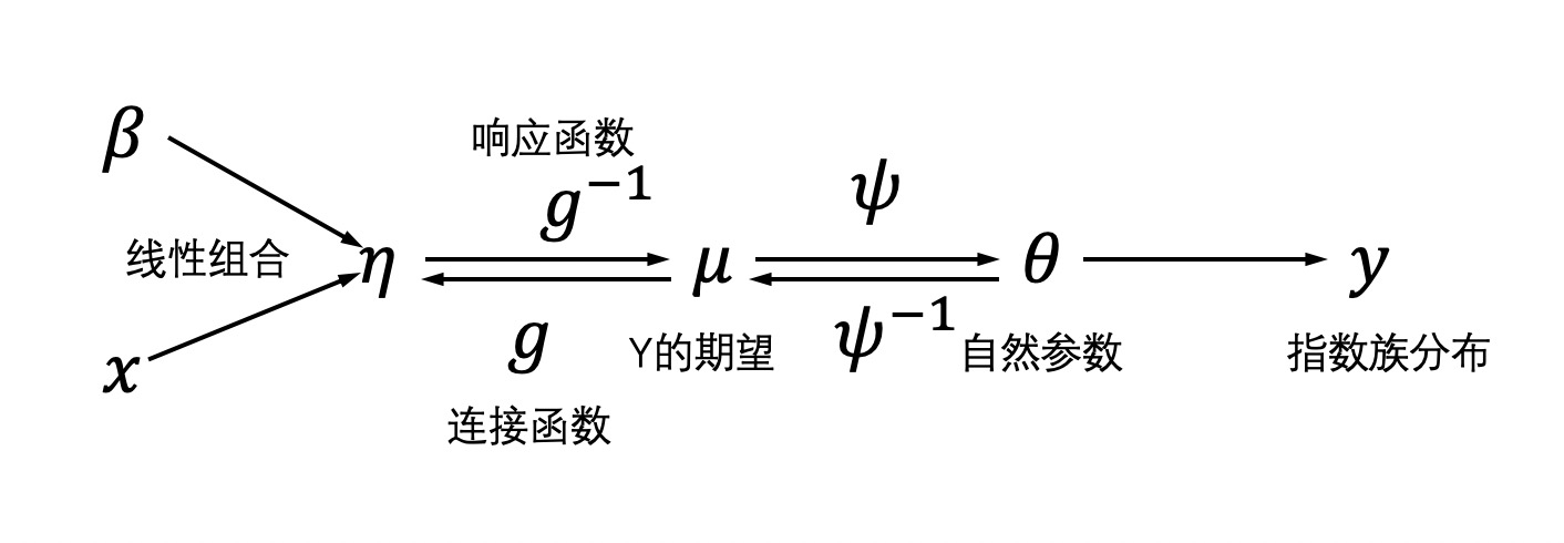
We know from the assumption that \(\theta\) is normally distributed and can be learned directly from the linear predictor. Thus, a good idea is to let \(g = \psi^{-1}\), so we have: \[ \eta = g(\mu) = \psi^{-1}(\mu) = \theta_\mu \] In this case, the \(\eta\) we are learning is exactly \(\theta_\mu\), which can be learned with a linear hypothesis space.

Hence, we we want to build a GLM to predict a variable \(Y|X \sim natural \ EFD(\theta)\)

1. Figure out the distribution type of Y, and rewrite it into a canonical form of EFD
2. Read \(\theta_\mu = \phi(\mu), b(\theta_\mu)\) out of the format and write down \(\mu = \psi(\theta_\mu)\)
3. Select the activation function as \(\psi^{-1}(\eta)\)
4. Train the model

The GLM enable us to generalize linear regression to many other cases, as long as Y|X follows a EFD. Common application includes Logistic Regression(Bernoulli Distribution), Softmax Regression(multi-category distribution), Polynomial Regression and so on. When Y|X follows a gaussian distribution, the activation function is just \(\mu = \eta\), and the model is reduced to a simply linear regression, which Y can be directly learned from a linear hypothesis space.

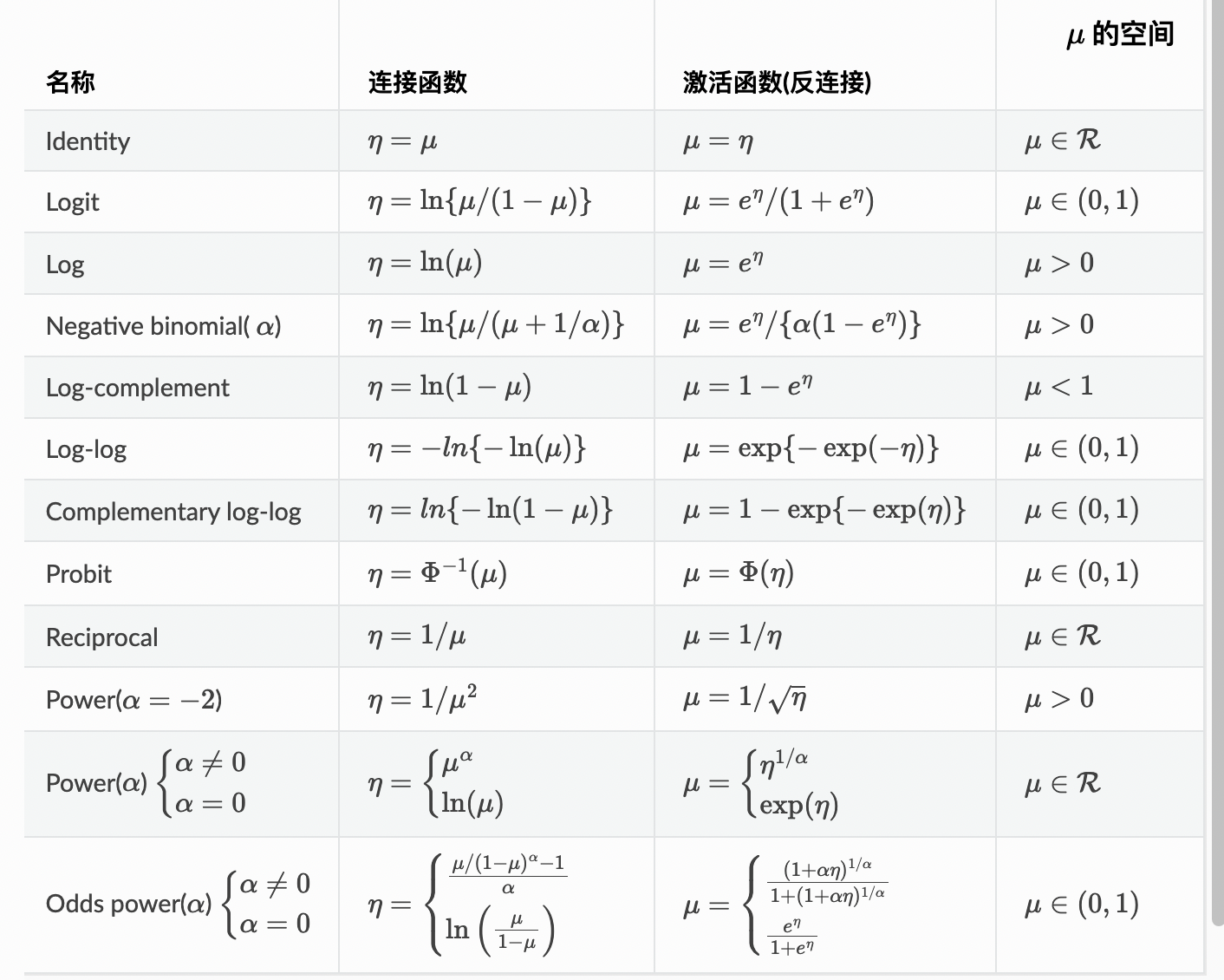
Some common joint functions and and activation functions are listed as follows: