A/B Testing: Experiment Sensitivity Improvement

1. About Sensitivity Improvement

If you expected there to be an significance effect but the results turn out to be insignificant, there's a chance that the sensitivity of the experiment is not big enough. In other word, given current sample size, your experiment can not perform enough statistical power as your demand. The sensitivity is usually measured by the Minimum Detectable E Effect(MDE).

Notice that when MDE is smaller than the PSB, even if we further improve the sensitivity by reduce mde, the mean of difference on metrics would still be lower than the PSB(any valid significant difference \(\mu\) should has \(\mu < mde\), while \(mde < psb\)). In such cases, the results have no chance to be practically significant. In other word, we only need improve sensitivity when: \[ MDE > PSB \] Recall the formula of MDE: $$ \[\begin{aligned} MDE &= (t_{\frac{1-\alpha}{2}} + t_ {1-\beta})SE[\delta]\\ &= (t_{\frac{1-\alpha}{2}} + t_ {1-\beta})\sqrt{V[\bar{Y_T}-\bar{Y_C}]}\\ & = (t_{\frac{1-\alpha}{2}} + t_ {1-\beta})\sqrt{V[\bar{Y_T}]+ V[\bar{Y_C}]}\\ &=(t_{\frac{1-\alpha}{2}} + t_ {1-\beta})\sqrt{\frac{\sigma_1^2}{n_ 1} + \frac{\sigma_2^2}{n_ 2}} \end{aligned}\]

$$ The formula suggests that if we want to maintain the desired statistical power, there are only two way to improve sensitivity:

More Sample

To collect more sample, we can:

• bring in more data by acquiring additional units
• increase test duration
• randomized on finer grain to increase sample size

Less Varaince

According to the equation of \(n', \delta, \beta\), we know that if the variance of the population is lower, we would need less sample to detect identical effect, given desired fixed statistical power, that is, the real-time statistical power would get higher while the sampe size remains the same.

In real application this can be difficult to implement extra sample acquisition. Thus, for this article, we focusing on techniques that can lowering the variance to improve experiment Sensitivity

2. Variance Estimation

Before lowering variance, first we need to make sure the variance of the parameters is estimated from the sample correctly. If the variance is incorrectly estimated, the p value and the confidence interval we calculated are both wrong.

When Randomized Unit \(\ne\) Analysis Unit

As discussed in this article, when estimating the standard error, we would usually assume the variable for the results of single units are i.i.d. However, such assumption are not always fulfilled. For example, there might exist network effects. We need to expel these effects before variance estimation

For some metrics like CTR, the unit is a pageview instead of a user. As multiple view can came from the same user \(B_1,B_2,..B_n\) may also be correlated. In thus case, we need to rewrite the metrics by aggregating it into a user level: \[ V[CTR] = V[\frac{user \ avg \ click }{user\ avg \ PV}] = V[\frac{\bar{X}}{\bar{Y}}] \]

When Using Relevant Difference(\(\Delta \%\))

Sometimes we would define the PSV using a relevant percentage instead of absolute value, like a 1% growth on GMV. In such case, we might want to judge the practical significance based on the confidence interval of a relevant of of the different between treatment and conrol group, let Y denote the measure on a single unit, \(\tilde{Y}\) denote the paramter to test on (mean or ratio), \(\Delta\) denote the difference of parameter between treatment and control group \[ \Delta\% = \frac{\Delta}{\tilde{Y_C}} = \frac{\tilde{Y_T}-\tilde{Y_C}}{\tilde{Y_C}} \] Thus, suppose \(\tilde{Y}\) is a mean parameter, when calculating the variance of \(\Delta\): \[ V[ \Delta] = V[\tilde{Y_T}-\tilde{Y_C}] = V[\tilde{Y_T}] + V[\tilde{Y_c}] = \frac{V[Y_T]}{n_1} + \frac{V[Y_C]}{n_2} \] However, when calculating the variance of \(\Delta\%\): \[ V[\Delta \%] = V[\frac{\tilde{Y_T}-\tilde{Y_C}}{\tilde{Y_C}}] = V[\frac{\tilde{Y_T}}{\tilde{Y_C}}] \] According to CTL, \(\tilde{Y_T},\tilde{Y_C }\) both follow normal distribution. Thus, the variance of \(\frac{\tilde{Y_T}}{\tilde{Y_C}}\) can be calculated from: \[ V[\Delta \%] = \frac{1}{\tilde{Y_C}^2}V[ \tilde{Y_T}] + \frac{\tilde{Y_T}^2}{\tilde{Y_C}^4} V[\tilde{Y_C}] + 2\frac{\tilde{Y_T}}{\tilde{Y_C}^3} Cov[\tilde{Y_T},\tilde{Y_C}] \] In a RCL, since treatment are randomly assigned, \(\tilde{Y_T}\) and \(\tilde{Y_C}\) are independent, thus \(Cov[\tilde{Y_T},\tilde{Y_C}] = 0\). Hence: \[ V[\Delta \%] = \frac{1}{\tilde{Y_C}^2}V[ \tilde{Y_T}] + \frac{\tilde{Y_T}^2}{\tilde{Y_C}^4} V[\tilde{Y_C}] \]

3. Metrics Manipulation

We can lower the variance by replace or transform the metrics

Metrics Replacement

Creating metrics with a smaller variance while capturing similar information. For example, the number of searches has a higher variance than the number of searchers; GMV has higher variance than order amount. The selection of lower-variance metrics should be validated in a real business environment.

Metrics Transformation

Transform the metrics so that it has lower variance. Common transformation includes discretization, log tranformation, and power transformation.

4. Construct Unbiased Estimator

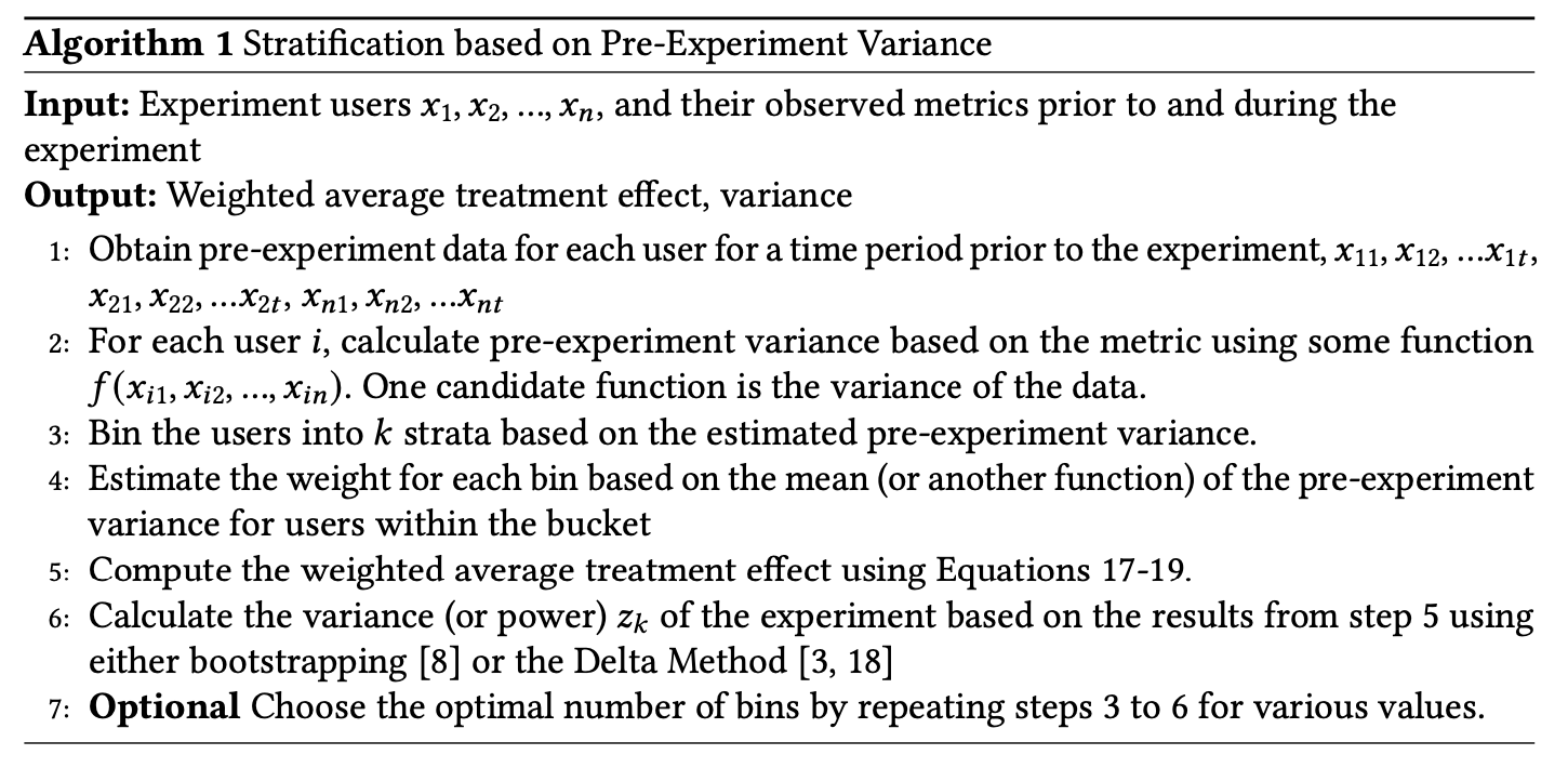
4.1 Stratification

In stratification, you divide the sampling region into strata, sample within each stratum separately, and then combine results from individual strata for the overall estimate by weighted sum, which usually has smaller variance than estimating without stratification.

Let \(Y\) be the value of the metrics(mean or ratio): \[ V[Y] = V[Y]_{within}+V[Y]_{between} = \sum_kp_k\sigma^2_k + \sum_kp_k(\bar{y}_k-\bar{y})^2 \] where \(p_k\) is the weight of the strata

Construct new estimator \(\hat{Y} = \sum_kw_kY_k\), where \(Y_k\) is the treatment effect of the \(k^{th}\) strata \[ V[\hat{Y}] = \sum_kp_kV[Y_k] = V[Y_{within}] < V[Y] \]

The stratification eliminate the between-group variance, thus can reduce the overall variance. However, the covariate, which is the strata, must be discrete.

Post-Stratification

While stratification is most commonly conducted during the sampling phase (at runtime), it is usually expensive to implement at large scale. Therefore, most applications use post-stratification, which applies stratification retrospectively during the analysis phase.

For post-stratification, we still conducted a randomized sampling to decided treatment group and control group. When analyzing the results, we put the units from treatment group and control group into buckets according to their strata variable with a ratio of 1:1. This saves the costs of doing multiple randomization, but it may waste a small portion of samples.

4.2 Regression Covariant Control

The covariate control method finds a continuous covariate that correlated with metric. The core idea is to make a regression relationship between the original metrics and its covariates. The covariates explain part of information of the original metric and contribute part of its variance. Thus, by taking out the part contributed by the covariate, the overall variance is lowered.

To some extent, the basic ideal of stratification and covariate control is the same. The difference is that covariate control method use regression to interpret the relationship between Y and its covariate.

Let X be the covariate. X should be constructed like the way Y does(mean or ratio). Construct new variable \(\hat{Y} = Y -\theta X\), if \(E[X_T] = E[X_c]\), then \(E[\hat{Y_T}-\hat{Y_C}] = E[Y_T-Y_c]\), the new variable is a unbiased estimation of the original metrics. It can be proven that \(V[\hat{Y}] < V[Y]\) if \(Cov[X,Y] > 0\).

Choosing Covariate

One thing to notice when choosing the covariate is that the assumption \(E[X_T] = E[X_c]\) should always be satisfied. Therefore, covariate should have no causal relationship with the experiment. If \(X \to T\), then the covariate is a confounder, then the covariate have different distribution on the treatment and control group,\(E[X_T] \ne E[X_C]\). On the other side, if \(T \to X\), then the X would be effected by the treatment, \(E[X_T] \ne E[X_C]\) after the experiment is conducted. Either way, the estimation is biased. Thus, when choosing covariates:

• The covariates should be pre-experiment metrics or invariant metrics that won't be affected by the experiment
• The covariates should be independent to the assigning of treatment and control group

A common application it to apply the same metric before the experiment as the covariate, as the pre-experiment metric is usually highly correlated with post-experiment metric. This method is usually called Controlled-experiment Using Pre-Experiment Data(CUPED)

Nevertheless, we can still used other covariate. Some thesis point out we can find such covariates through machine learning methods. These methods includes CUPAC(Control Using Predictions As Covariates) and MLRATE(machine learning regression-adjusted treatment effect estimator)

Controlled-experiment Using Pre-Experiment Data(CUPED)

Let X denots the value of the metric we want to test before the experiment, Y denots the value after the experiment. For an A/B test, we expect that \(E[X_T] = E[X_C], E[Y_T] \ne E[Y_C]\). Now construct two variables: \(\hat{Y_T} = Y_T - \theta X_T\), $ = Y_C - X_C$, where \(\theta\) is a hyperparameter we can adjust. We know that: \[ E[ \hat{Y_T}-\hat{Y_C}] = E[(Y_T - \theta X_T) - (Y_C - \theta X_C)] = E[Y_T]-E[Y_C] \] thus, estimate the treatment effect on CUPED variable is equivalent to estimate the effect on original metrics. Meanwhile: \[ V[\hat{Y_T}-\hat{Y_C}] =V [(Y_T - \theta X_T) - (Y_C - \theta X_C)] = V[Y_T- Y_C] +\theta^2V[X_T-X_C]-2\theta Cov[(Y_T-Y_C),(X_T-X_C)] \] we can than regard \(V[\hat{Y_T}-\hat{Y_C}]\) as a quadratic function of \(\theta\), where: \[ \Delta = 4Cov[(Y_T-Y_C),(X_T-X_C)]^2 - 4V[(Y_T - Y_ C)]V[X_T-X_C] \] as we know: \[ Cov[X_1,X_2] \le \sqrt{V[X_1]V[X_2]} \] we have that \(\Delta \ge 0\), thus: \[ V[\hat{Y_T}-\hat{Y_C}] \in [0,V[Y_T- Y_C]] \qquad \theta \ge 0 \] we have minimum \(V[\hat{Y_T}-\hat{Y_C}]\) when \(\theta =\frac{Cov[(Y_T-Y_C),(X_T-X_C)]}{V[X_T-X_C]}\)

4.3 Variance-Weighted Estimators

For a single user, we can write the outcome of his experiment results of metrics Y as: \[ Y = \alpha+ \delta _iZ_ i +\epsilon_i \] where \(\alpha\) is the basic level of the outcome, \(\delta_i\) is the treatment effect on the \(i^ {th}\) user, \(Z_i\) is a indicator of whether that user are exposed with the treatment, and \(\epsilon_i\) is the random error of his observation. Suppose \(\epsilon_i \sim N(0,\sigma_i^2)\), then \(V[\delta_i] = \sigma_i^2\). This means the variance of treatment effect on a single user is decided by the characteristics of that user. We typically assume homogeneity in the variance of the error terms \(\sigma _i^2 = \sigma^2\), in other world, we treat all user as identical person except for whether they are exposed with the treatment. However, it is totally sensible if different user's variance are naturally different.

Like the idea of stratification, we can regard the total variance as: \[ V[\delta] = E_i[variance \ of \ user \ i]+ E[variance \ among \ users ] \] Thus we can let: \[ \hat{ \delta} = \sum_i w_ i\delta_ i \] With derivation, it can be proven that when we set: \[ w_i = \frac{\sigma^2_i}{\sum_i\frac{1}{\sigma^2_i}} \] we would have lowest variance: \[ min \ V[\hat{\delta}] = \frac{1}{\sum_i\frac{1}{\sigma_i^2}} \] here: \[ \begin{aligned} V[\delta]-V[\hat{\delta}] &= \frac{\sum_i\sigma_i^2}{n} -\frac{1}{\sum_i\frac{1}{\sigma_i^2}} \\ & = \frac{\sum _i\sigma^2_i\sum_i\frac{1}{\sigma_i^2} - n}{n\sum_i\frac{1}{\sigma_i^2}}\\ & >0 \end{aligned} \] Thus, we lower the variance of the treatment \(\bar{Y_T}-\bar{Y_C}\) and thus lower the MDE, increase the sensitivity of the experiment.

In real application, \(\sigma_i^2\) are estimated from pre-experiment data of Y on user i. For cost-saving calculation reason, we would bin the users into K groups and use the mean of user's variance who is in the group: \[ w_k = \frac{1}{\sigma_k^2} = \frac{1}{\frac{1}{n_k}\sum_{i \in k}\sigma_i^2} \]

5. Triggering Analysis

5.1 Triggering

Triggering provides experimenters with a way to improve sensitivity (statistical power) by filtering out noise created by users who could not have been impacted by the experiment. As organizational experimentation maturity improves, we see more triggered experiments being run.

If you make a change that only impacts some users, the Treatment effect of those who are not impacted is zero. This simple observation of analyzing only users who could have been impacted by your change has profound implications for experiment analysis and can significantly improve sensitivity or statistical power.

Commonly triggering analysis can be applied in the following situations:

1. Intentional Partial Exposure: The treatment are designed to take effect on only some particular population. For example, a new UI are only exposed to Android user. Note that if there exists some “mixed” population, in this case, users that log on both Android and IOS, then these user should also be regarded as observation population
2. Conditional Exposure: the change is to users who reach a portion of your product. For example, we improve the payment procedures, but users need to reach the checkout page to experience the new procedures
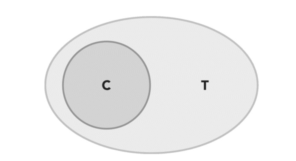
3. Coverage Increase: The strategy of the treatment group covers the strategy of the control group. For example, in control group, we offer users buy more than $30 with free shipment fee, while in treatment group, we lower the threshold to \(20 dollars. In this case, the treatment strategy totally cover the control group, the overlapping population(\){T C}$), which is users buy over $30, are supposed to have zero effect and thus should not be triggered. Samely, those who buy under \(20(\){U-(TC)}$) shoule not be triggered. Only those who buy between $20 and \(30(\){T-C}$) should be triggered

1. Coverage Change: the coverage isn’t increased, but is changed, as shown in the Venn diagram. For example, Control offers free shipping to shoppers with at least $30 in their cart but Treatment offers free shipping to users with at least $20 in their cart except if they returned an item within 60 days before the experiment started. In such case, the population should be triggered are those who
   1. \(\{T-C\}\): buy between $20 and $30 and do bot return any itemsin 60 days,
   2. \(\{C-T\}\): those who buy over $30 but return items in 60 days

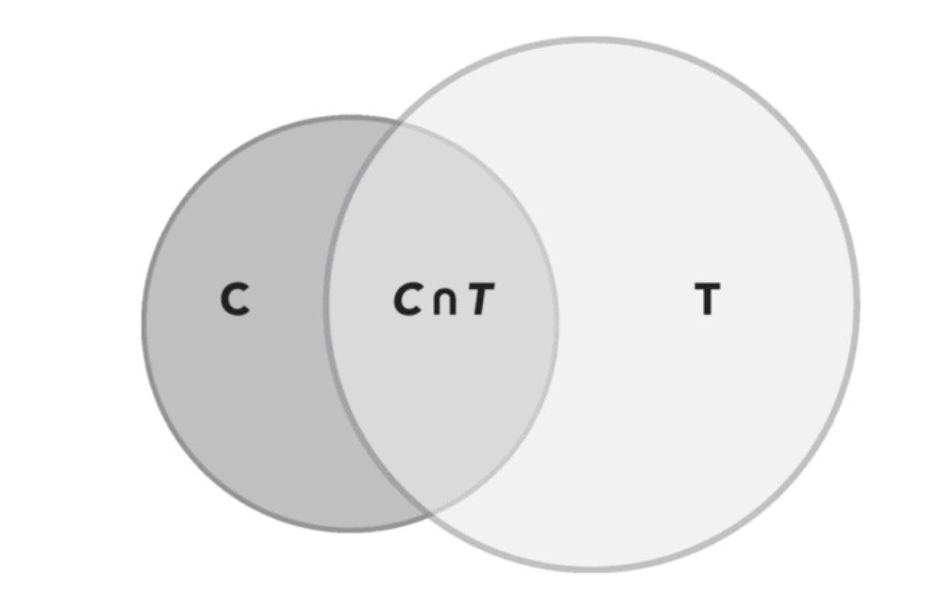
note that the same metric can go opposite on these two parts, and neutralized the overall effect.

Optimal and Conservative Triggering

When comparing two variants, the optimal trigger condition is to trigger into the analysis only users for which there was some difference between the two variants compared. In other word, the counterfactuals of that user would be different.

In practice, however, we sometimes need to include more users than the optimal triggering population:

1. Multiple Treatment: When there exists multiple treatment, a sub population that is assumed to have zero effect between \(C\) and \(T1\) may have differences between \(C\) and \(T2\):

\[ \begin{aligned} Y_{sp}(T1) - Y_{sp}(C) &= 0\\ Y_{sp}(T2) - Y_{sp}(C) &\ne 0 \end{aligned} \]

2. Lack of samples: Sometimes triggering analysis would significantly reduce the number of samples. A low number of samples can also decrease statistical power. In this case, we consider expanding the triggering population to achieve the optimal balance of statistical power.

3. The recognition of optimal triggering population is unavailable: For example, the treatment is improvement procedure, but the event tracking for entering checkout page is missed. In this case, we can enlarge the population to “user who click the checkout button in shopping car page”

5.2 Pitfalls in Triggering Analysis

Triggering is a powerful concept, but there are several pitfalls to be aware of.

Estimating Overall Effect

Suppose the triggering population accounts for 10% of the volume and we detect a 3% improvement on some metrics. Does that mean the overall effect is 0.3%? The answer is no. Actually, the real effect can be any number between 0% and 3%, or even negative.

For example, the treatment is to improve the payment procedures and the triggering population is those who reach the checkout page. We observed a 3% improvement on revenue. One fact is, only those who reach the checkout page can produce revenue, so the real effect on the overall population can still be 3%. Triggering analysis only lower the variance by conditioning on a sub population and thus make the difference statistically significant.

Oppositely, if the triggering population are some low-spending user, then the real overall effect can also be much lower than 0.3%. Only when the metric have the same distribution on the overall population and the sub population, can we estimate the overall treatment effect simply based on sub population ratio.

Besides, there can also be a Simpson paradox and drive the overall effect to the contrary side. For example, in the former example, the treatment may enlarge the ratio of the low-spending population and cause the decrease of overall revenue, even when the conditional effect on the triggering population is positive

Experimenting on Tiny Segments That Are Hard to Generalize

The triggering population should somehow be representative, or we can say, meaningful. In the case of improving payment procedures, even though the users who reach the checkout page only account for 5% of the total users, they may contribute more than 99% of the revenue. In this scenario, conducting a triggering analysis based on the revenue metric is reasonable.

However, let's consider a different scenario where the treatment involves highlighting the first video on a video searching page, and we only trigger for users who click on the first video. In this case, the best conclusion we can draw is that "highlighting the first video improves its play times." It may be difficult to generalize this conclusion to all videos on the searching page, as different videos naturally have varying play amounts, and the first video represents only a small portion of all the videos.

The selection of triggered user are influenced by the treatment itself

Theoretically, we should guarantee the treatment itself does not change the selection of triggered users. For example, in the case of improving payment procedures, the triggered users are those who who reach the checkout page. However, the new procedures are so terrible that many users do not click the checkout button and enter the checkout page again. If we still focus only on those who reach the checkout page, we may found the average revenue of them does not drop significantly, but the real effect is underestimated.

In real application, when the treatment has a causal effect on the probability that a unit is triggered, unexpected dependence can be introduced. A solution is to keep a user in the population for analysis once he is triggered.