Probability Density Estimation

1. About Probability Density Estimation

Probability Density Estimation(PDE) is a techniques used for estimating probability distribution of a variable through samples. Specifically, it can be categorized as:

• Parameter Estimation: Assuming the variable follows a type of distribution and estimating the parameter of that distribution through samples
• Non-parameter Estimation: Trying to obtain the distribution of the variables directly from the data without any distribution type assumptions

For PDE, we usually assume that all samples are i.i.d

2. Parameter Estimation

2.1 Maximum Likelihood Estimation

Consider the Bayesian's Law: \[ P(X=x|Y=y) = \frac{P(Y=y|X=x)P(X=x)}{P(Y=y)} \] One critical thing to remember is the way to interpret the parameter \(\theta\).

According to Bayesian, the parameter \(\theta\) itself sollows some kinds of distribution. Thus, the likelihood and posterior distribution in bayesian's law is exchangeable, \(\theta\) is nothing but a random variable just like X and Y in equation 1. In such scenarios, likelihood and probability is the same thing \[ P(\theta|E) = \frac{P(E|\theta)P(\theta)}{P(E)} \] where E represents the evidence variable.

However, according to frequentist, \(\theta\) is a unknown constant values, and it does not have a distribution. Thus, there's \(\theta\) cannot be put into the Bayesian's Law like a random variable. In this scenario, likelihood and probability is not one thing. Probability is for random variable, while likelihood is for parameter, which is a constant values. According to frequentist, given the i.i.d. assumption: \[ L(\theta| D) = P(D|\theta) = \prod_iP(d_i=x_i|\theta) \] where D represents the results of all samples.

The MLE is a product of the frequentist. Thus, in MLE, to find best \(\theta\), we just need to find the \(\hat{\theta}\) that maximize the likelihood function. For calculation, do average log operation on both sides: \[ \iota(\theta|D) = \frac{1}{n}lnL(\theta| D) \]

\[ \hat{\theta} = argmax \ \iota(\theta|D) \]

The best parameter \(\theta\) can thus be obtained calculating the zero point of the derivation function of the \(\iota(\theta|D)\)

2.2 Bayesian Estimation

The Bayesian is the other side of view on probability. According to format (2): \[ P(\theta|E) = \frac{P(E|\theta)P(\theta)}{P(E)} = \frac{P(E|\Theta = \theta)P(\Theta = \theta)}{\sum_i P(E|\Theta =\theta_i)P(\Theta=\theta_i)} \] In this equation:

• \(P(\theta)\) follows the prior distribution, which is decided by prior knowledge regardless of the sample information
• \(P(E|\Theta=\theta_i)\) is the likelihood function decide by the knowledge of the mechanism between \(\theta\) and \(E\) regardless of sample information

The bayesian estimation is a process of updating the prior knowledge through sample information. The updated posterior distribution can be the new prior distribution. In real application, the accurate understanding of the likelihood function can be difficult, besides, the calculation can also be quiet difficult.

2.3 Maximum A Posterior Estimation

The Maximum A Posterior Estimation is an approximation of the bayesian estimation. it assume the marginal distribution \(P(E)\) is independent of the parameter distribution \(P(\theta)\). It calculate the best \(\theta\) by maximize the posterior probability \(P(\theta|E)\) \[ \hat{\theta} = argmax \ f(D|\theta)g(\theta) = \prod_iP(d_i=x_i|\theta)P(\theta) \] Such assumption make the calculation of the posterior probability much more easier. The MAP allows to add the prior distribution of \(\theta\) into the estimation. It is a simpler version of Bayesian Estimation.

3. Non-parameter Estimation

3.1 Histogram

A histogram is a graphical representation of data distribution. It is used to show the frequency distribution of a set of continuous or discrete data. In a histogram, the data is divided into a set of intervals, also known as bins. The number of values that fall into each bin is represented by the height of the bar above the bin.

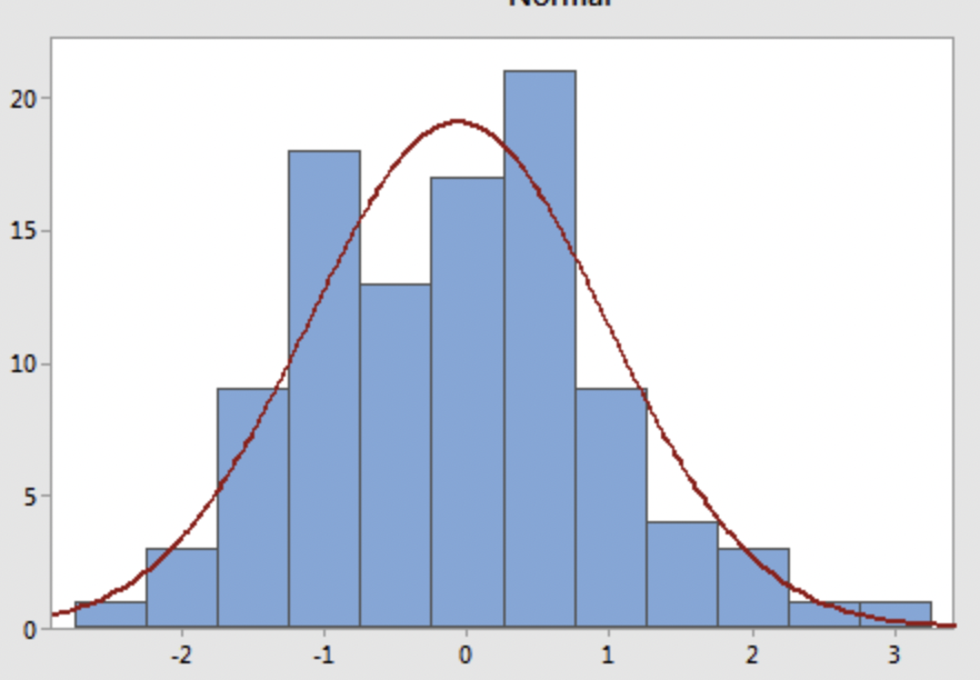
Let \(h\) denote the width of a bin with range \([a,a+h]\), Let \(k\) denote the number of sample in that bin, n denote the total number of samples. The probability density in any points lie in \([a, a+ h )]\) would be: \[ P(x) = \frac{k}{nh} \]

There is no optimal method for selecting the bin width of a histogram. A bin width that is too large can distort the estimated probability distribution, while a bin width that is too small can lead to overfitting. In addition, the probability density estimated from histogram are not continuous on the endpoints on bins. Therefore, histograms are often only used to roughly observe the shape of a distribution and cannot be used for accurate probability predictions.

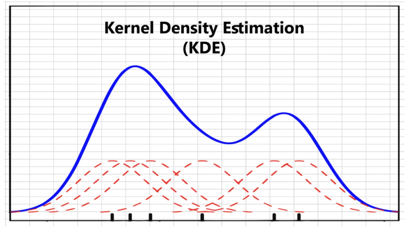
3.2 Kernel Density Estimation(Parzen Windows)

KDE can be seen as a improvement of histogram. We know that PDF is the derivative of CDF. For a histogram, when the value of \(h\) tends to 0, we obtain the PDF. Let \(f(x)\) denote the PDF and \(F(x)\) denote the CDF: \[ f(x) = \lim_{h \to 0} \frac{F(x+h) - F(x-h)}{2h} \]

In a histogram, we use the empirical distribution, which is the ratio of the number of data points falling in the interval \([x-h, x+h]\) to the total number of data points, to substitute \(F(x+h) - F(x-h)\). By taking a small enough \(h\) to ensure that the condition \(h \to 0\) is satisfied, we obtain the probability density formula for the histogram:

\[ p(x) = \frac{count_{x_i}([x-h,x+h])}{2nh} \]

Now, we assume that the data points falling within the interval \([x-h,x+h]\) have different contributions (weights) to the probability density estimate of \(x\). This contribution satisfies a certain distribution, where the farther away from \(x\), the smaller the contribution, and the integral should be equal to 1. We use a function \(K(\frac{x_i-x}{h})\) to represent the contribution of data point \(x_i\) near \(x\) to \(p(x)\), and let \(t = \frac{x_i-x}{h}\), \(K_0(t) = \frac{1}{2}K(t)\), ensuring that \(\int K_0(t)dt = 1\). At this point, the PDF estimate becomes:

\[ p(x) = \frac{1}{2nh}\sum_{x_i\in [x-h,x+h]} K(\frac{x_i-x}{h}) = \frac{1}{nh}\sum_{x_i\in [x-h,x+h]} K_0(t_i ) \]

At this point, we refer to \(K_0(t)\) as the kernel function and the estimation of \(p(x)\) as kernel density estimation. The estimation of \(p(x)\) is continuous, meaning that for any \(x\), we can estimate the corresponding \(p(x)\), unlike histograms where the probability density estimation of bin endpoints is discontinuous.

Common kernel functions for KDE includes:

• Gaussian kernel: \(\phi(t) = \frac{1}{\sqrt{2\pi}}e^{-\frac{1}{2}t^2}\)
• Exponential kernel: \(\phi(t) = e^ {-|u|}\)
• Triangular kernel: \(\phi(t) = \left \{ \begin{aligned} &1-|t| \quad &|t|<1\\ &0 &otherwise \end{aligned}\right.\)
• hypersphere kernel: \(\phi(t)= \left \{ \begin{aligned} &1 \quad &||t||<1\\ &0 &otherwise \end{aligned}\right.\)

When we adopt the hypersphere kernel, the contribution function works the same as the counting in the histogram, the difference is that instead of pre-decide all sections, we now count the the points in section \([x- h,x+ h ]\) for any \(x\) , so \(p( x )\) is continuous. Just like histogram, the KDE still need us to manually decide \(h\) , and the trade-off between distortion and overfitting still exists.

3.3 K Nearest Neighbors

KDE fixed the length \(h\) of the neighborhood of \(x\). This approach may lead to unstable estimation results of probability density for some regions with low density, where there are very few data points within the neighborhood of \(x\). As an alternative approach, we can fix the number \(k\) of data points within the neighborhood of \(x\) and allow the length \(h\) to vary. In this case, the estimation of probability density is given by:

\[ p(x) = \frac{k}{nV_k(x)} \]

where \(V_k(x)\) is the length of \(x\)’s neighborhood that contain \(k\) neighbors.