A/B Testing: Results Analysis

1. Sanity Check

After we obtained the results data and before we make any analysis, we want to do some sanity check to ensure the experiment are running correctly and any differences are caused by the treatment instead of any other changes. A Sanity check refer to the simple process to verify the resutls by checking the consistency of those metrcis that are not supposed to be affected by the treatment(Invariant Metrics). There are two types of invariant metrics:

1. Trust-related guardrail metrics: Metrics related to the business process but should not be effected by the treatment or should be configured the same for both group(e.g search amount for a watch-time duration test, cache hit rate, Telemetry fidelity)
2. Organiztional guradrail metrics: metrics that are important to the organization and expected to be an invariant for many experiments.(e. g. latency, GMV, PV)

If these sanity checks fail, there is probably a problem with the underlying experiment design, infrastructure, or data processing.

2. Judgment on Significance

2.1 Judgement on Statistical Significance

The judgement on statistical significance should be based on p value calculated from the test results.

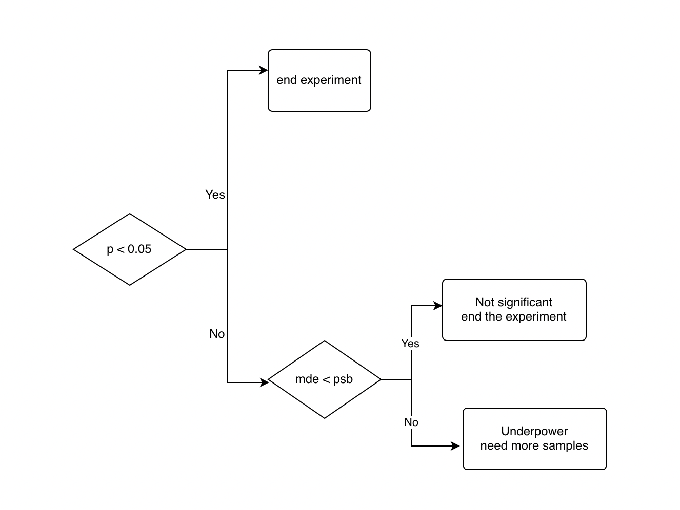
Note that the MDE is the real-time sensitivity estimated from the experiment results

2.2 Judgement on Practical Significance

Confidence Interval

From a frequentist probability theory POV, the confidence interval is a section describe how often the true value of a parameter would lie in the section given a significance level. In a testing we regard the observed difference as an estimation of the mean of the true difference, following a normal distribution. We can then calculated the CI through: \[ CI = [\mu- Z_{\frac{\alpha}{2}}*\sigma_{SE},\ \mu+ Z_{\frac{\alpha}{2}}*\sigma_{SE}] \] where:

• \(\mu\) is the observed difference
• \(\sigma_{SE}\) is the standard error estimated from the standard deviation from the sample

Practical Significance

When checking on CI, the following situations may occur:

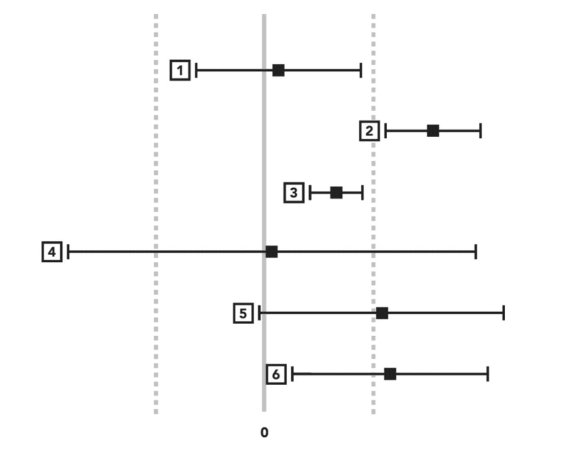
1. The result is not statistically significant. It is also clear that there is no practical significance. This suggests that the change does not do much. You may either decide to iterate or abandon this idea.
2. The result is statistically and practically significant, which suggests lauching the feature.
3. The result is statistically significant but not practically significant. In this case, you are confident about the magnitude of change, but that magnitude may not be sufficient to outweigh other factors such as cost and thrive you business goal.
4. The boundry of the CI does exceed the PSB but it happens in both way. This ethier suggest the treatment effect is very unstable or the experiment is underpowered. Consider running a follow-up test with more units, providing greater statistical power
5. The result is likely practically significant but not statistically significant.There is a good chance that there is no impact at all. From a measurement perspective, the best recommendation would be to repeat this test but with greater power to gain more precision in the result.
6. The result is statistically significant, and likely practically significant. There is still a chance that the impact is not sufficient from a business perspective. While we still should consider repeating the test with more power, choosing to launch is a reasonable decision from a launch/no-launch decision

From the analysis above we found only scenarios 2 and 6 could be considered launchable. Whether we should stick to scenario 2 depends on our preference. In most business practice we would presue scenario 2.

2.3 Judge of Significance in Multiple Testing Scenarios

2.3.1 Multiple Testing Scenarios

Multiple Variants

There are more then two variants. For example, suppose we want to examine the imporvement on CTR by changing the color of a button, but we have three alternative treatments. In this case we creat three tests. For each test, let \(\alpha = 0.05\), then: \[ P(no\ false \ positive \ in \ all \ three \ tests) = (1-\alpha)^3 = 0.857 \] The type I error of the overall experiment hypothesis, which is "changing color improves CTR" is high.

Multiple Metrics

Suppose we have only one 1 treatment but 100 metrics to test. Set \(\alpha = 0.05\), same as the multiple variants scenario, around 5 metrics would fall into the pitfall of type I error, which means they will be false positive, and this could mislead.

2.3.2 Corrections of Significance Level under Multiple Testing

Bonferroni Correction

Bonferroni Correction is a simple way to lower type I error by having smaller \(\alpha\) for each test: \[ \alpha_i = \frac{\alpha}{n} \] where n is the number of tests(number of variants, number of metrics, or the product of them)

The bonferroni correction is easy to apply, but it is also to conservative. It increase the difficulty to reject the null hypothesis in each test.

Control False Discovery Rate

Define FDR as: \[ FDR = E[\frac{n_{FP}}{n_{rej}}] \] FDR tells in all tests that we judge as significant, how many of them are false positive. For example, suppose we have 1000 testing and reject 200 of them, and the FDR = 0.05, then we can expect around 10 metrics to be false positive. If we take this results as acceptable, we can move on to analysis. Otherwise, we should consider lower \(\alpha\)

In real application, the judgement of false positive can be difficult to detect. Thus, controlling PDR can be sometimes unaccessible.

Benjaminiand Hochberg's Method

Suppose we have n tests, each has a p value as a result. First, we can rank the list in a ascending order by P values. Then we correct the p value with: \[ q_i = p_i * \frac{n}{k} \] Where k is the ranking of the \(i^{th}\) test

T	P value	Q
T2	0.001	0.005
T5	0.003	0.0075
T1	0.12	0.4
T3	0.045	0.54
T4	0.048	0.048

we then comepare the Q value with \(\alpha\) to judge the significance.

This process can lower the overall type I error. However, we may also notice that through this method, alternatives with greater p value can pass while alternatives with smaller p values can fail, which sometimes may mislead.

Two-step Rule-of-thumb

Another method when dealing with multiple metrics is to segment the metrics in serval tiers, such as:

• First-order metrics: those you expect to be impacted by the experiment
• Second-order metrics: those potentially to be impacted
• Third-order metrics: those unlikely to be impacted

and apply tiered significance levels to each group (e.g., 0.05, 0.01 and 0.001 respectively).

3. Validity Check(Truthworthyness Analysis)

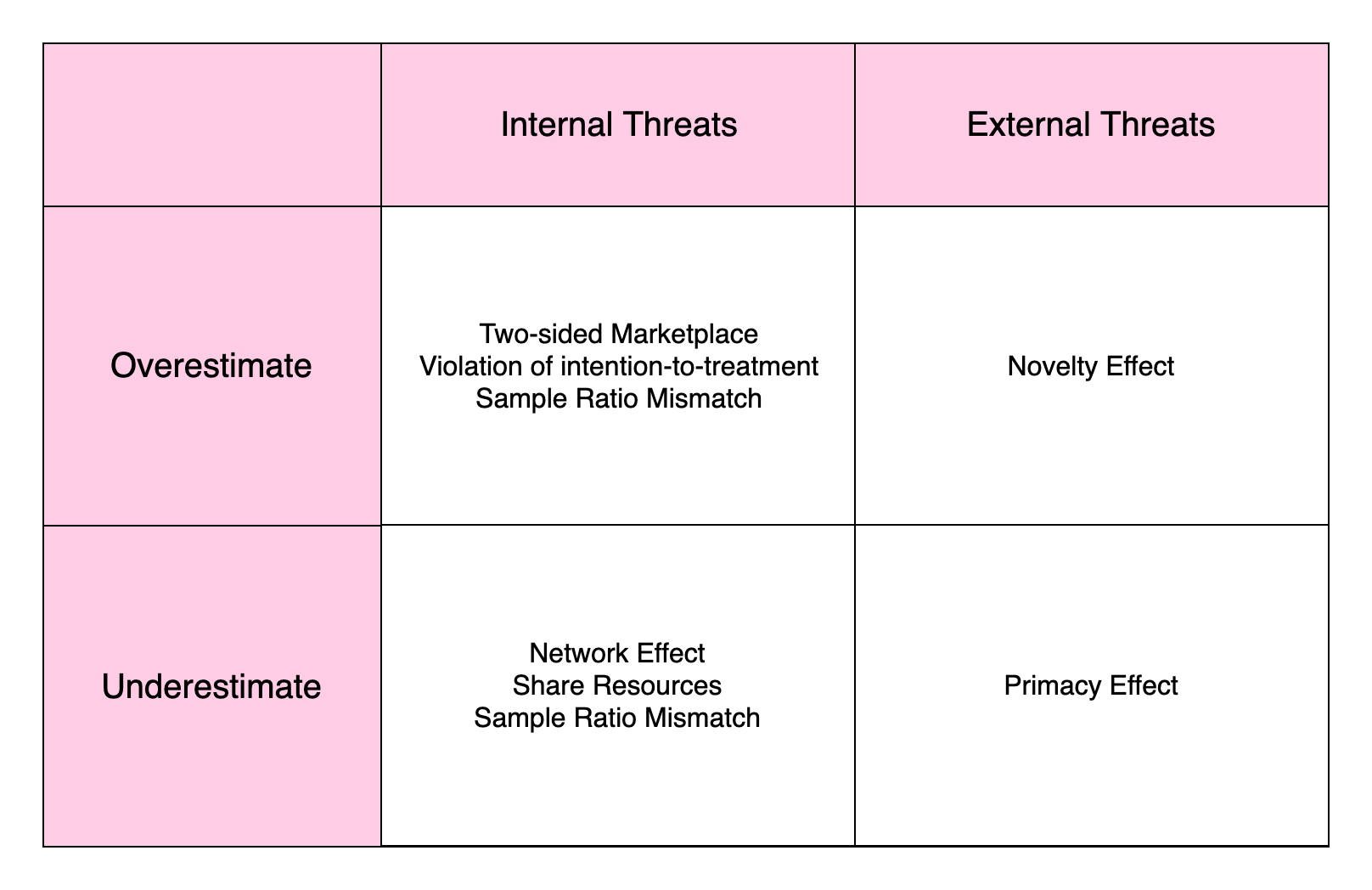
The Validity Check is a process is a procedure to find out if the results are truthworthy. It is usually an analysis to rule out some potential effects that could threat the validity. Such analysis can be decomposed on two dimensions:

Internal Threats/External Treats:

• internal: Making the testing results itself is incorrect without attempting to generalize the results to other population or time periods
• external: Making the conclusion incorrect when trying to generalize it to other population or time periods

Overestimate/Underestimate

• Overestimate: The testing results is significant but the real effect or generalized effect is not so
• Underestimate: The testing results is insignificant but the real effect or generalized effect is not so

3.1 Threats to Internal Validity

3.1.1 Violation of SUTVA

A random controlled experiment requires Stable Unit Treatment Value Assumption (SUTVA). It states that experiment units (e.g., users) do not interfere with one another. In some cases, this assumption could be violated

Network Effect

A feature might spillover to other user through the social network of treatment unit. This usually undermine the difference between control and treatment group. If the treatment is applied to all users, the real effect can be bigger. To deal with this kind of effects, we can implemented social network clustering and select randomized unit for control and treatment group in different clusters. There is also a method called ego-network randomization

Two-sided marketplaces: For two-sided platform like auctions platform or Uber. The treatment on the unit might affect other unit through the "other-side". For example, lowering prices for riders in Treatment group make them more attractive to drivers, and there would be less drivers available for control group. In this case, the GMV difference between two groups are overestimated. The real differences between when the treatment applied to all users might be lower. To deal with this kind of effects, we can make geo-based or time-based isolation on treatment and control group

Shared Resources: If the Treatment leaks memory and causes processes to slow down due to garbage collection and possibly swapping of resources to disk, all variants suffer.This could lead to underestimating of real effect. For example, the Treatment crashed the machine in certain scenarios. Those crashes also took down users who were in Control, so the delta on key metrics was not different —both populations suffered similarly.

3.1.2 Violation of Intention-to-Treatment

In an online experiment, the treatment group shoud be those whose treatment are "delivered" rather than "fulfilled". Our measuring is based on the offer, or intention to treatment, not whether it was actually applied. Analyzing only those who participate, results in selection bias and commonly overstates the Treatment effect. For example, if our treatment is "adding an subscribe button" and our target is to increase revenue, then our treatment group should be those who are demonstrated with the button instead of those who actually click the button. We can add a second success metric "CTR" to track the effectiveness of the button though.

3.1.3 Sample Ratio Mismatch

If the ratio of users (or any randomization unit) between the variants is not close to the designed ratio, the experiment suffers from a Sample Ratio Mismatch (SRM). A SRM indicates the decision of exposing a unit to the treatment is not independent to treatment effect. This could lead to either overestimate or underestimate.

For example, the ratio designed for treatment and controlled group is one-to-one. Suppose the decision is randomly obtained through a coin flip, then the expected sample ratio should be 0.5. We can regard the sample ratio as a parameter and test it if through t distribution. If the p value is samll enough, we can make the claim that there's some problem with the coin that lead to a sample ratio mismatch.

The cause of the SMR, in most cases, is for the developer to worry. Debugging SRMs requires the developer to examine their randomization strategy during experiment configuration.

3.2 Threats to External Validity

3.2.1 Primacy and Novelty Effect

Primacy Effect: When a change is introduced, users may need time to adopt, as they are primed in the old feature, that is, used to the way it works. In other word, users are reluctant to changes. This effect would diminish over time, but if we made the conclusions while the primacy effect still exists, than we may underestimate the real treatment effect

Novelty Effect: Being opposite to the primacy effect, the novelty effect refer to that a new feature might be attractive for the users at first, but not so interesting after the users try them for the first time. This effect would diminish over time, but if we made the conclusions while the novelty effect still exists, than we may overestimate the real treatment effect

Solutions for these two effects:

• ensure the experiment run long enough so that these two effects vanish over time
• rule out these effects by constraining the target group in only first-day user
• compare the CATE of first- time and existing user to see if the effects do exist

4. Segmentation Difference & Outlier

4.1 Segmentation Analysis

Analyzing a metric by different segments can provide interesting insights and lead to discoveries. Things we can do about segmentation includes:

Segmental View on Metrics: Inspecting the segmentation metrics values before and after the experiment. If the metrics are distinctly different for a group, then this group may have a strong difference comparing to other groups. We can dive in to the problem and make debugging or take this group out of the target group

Segmental View on Effect: Inspecting the CATE of the segmentations. For any strongly distinct CATE, we can doubt that the treatment takes effect with a special mechanism on this particular group. We can dive in to the problem and make debugging or take this group out of the target group

Migration Among Segmentations :

Suppose we want to examine the improvement of CTR of users brought by a treatment. We find the CTR of treatment and control group are respectively 25 v.s. 20 for Chinese users, and 15 v.s. 10 for non-Chinese users .Can we know make the conclusion that the treatment is effective?

The answer is no. We need to first ensure there are no unit migrations among segmentation. If the assignment of the feature make some chinese decide to change their language options and turn them to non-Chinese users. The overall treatment effect may go down

This indicates that analysis on segmentations can mislead due to migration. The segmentation should be done based on the status of units before the experiment. Otherwise, migrations among groups can happen

4.2 Outlier Influence

The existence of outliers can drastically change the conclusion regarding significance.

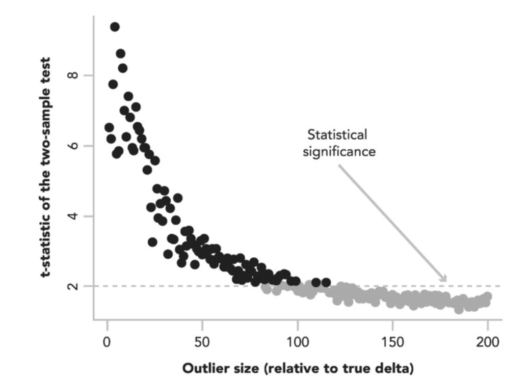
Thus, it is necessary to eliminate the outliers in the samples before making conclusions. For example, a user who has 10000 pageviews is probability a robot. For outlier detection techniques, refer to this article.

5. Improvement of Experiment Sensitivity

5.1 Sensitivity Improvement

For sensitivity improvement methods, refer to this article