Probability Graphical Model

Probability Graphical Model: Basis

1. About Probability Graphical Model

The Probability Graphical Models are a series model that express the dependency/ joint distribution in a graphic way(edges and nodes). The apllications of PGM includes:

• PGM representation: present the correlation or causality relationship among variables in a graphical way
• PGM learning: including parameter learning and structural learning
• PGM inference: reasoning the correlation/causality structure of variables

2. Terminology

Factor

A factor is a funtion of one or more variables \[ \phi(X_1,..X_n) \] where \(\phi: Val(X_1,...X_n) \to R\)

Scope

The list of variables included in a factor: \(\{ X_1, ...X_n\}\)

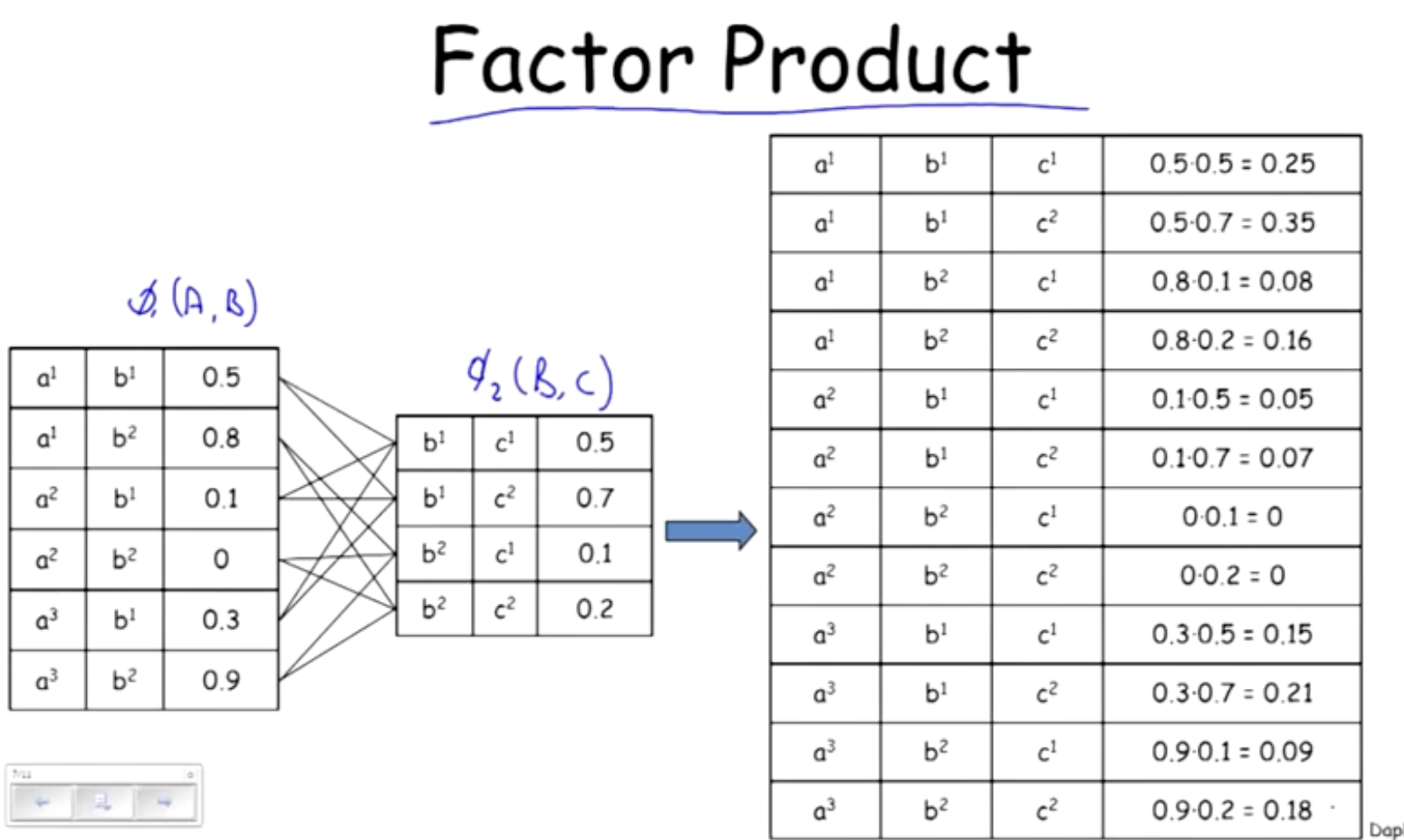
Factor Product

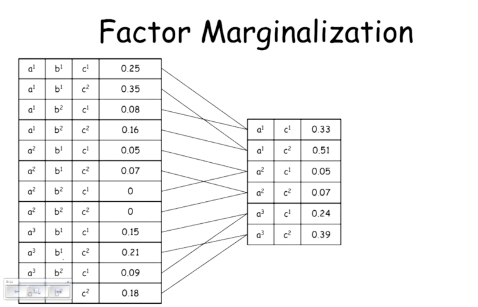
Factor Marginalization

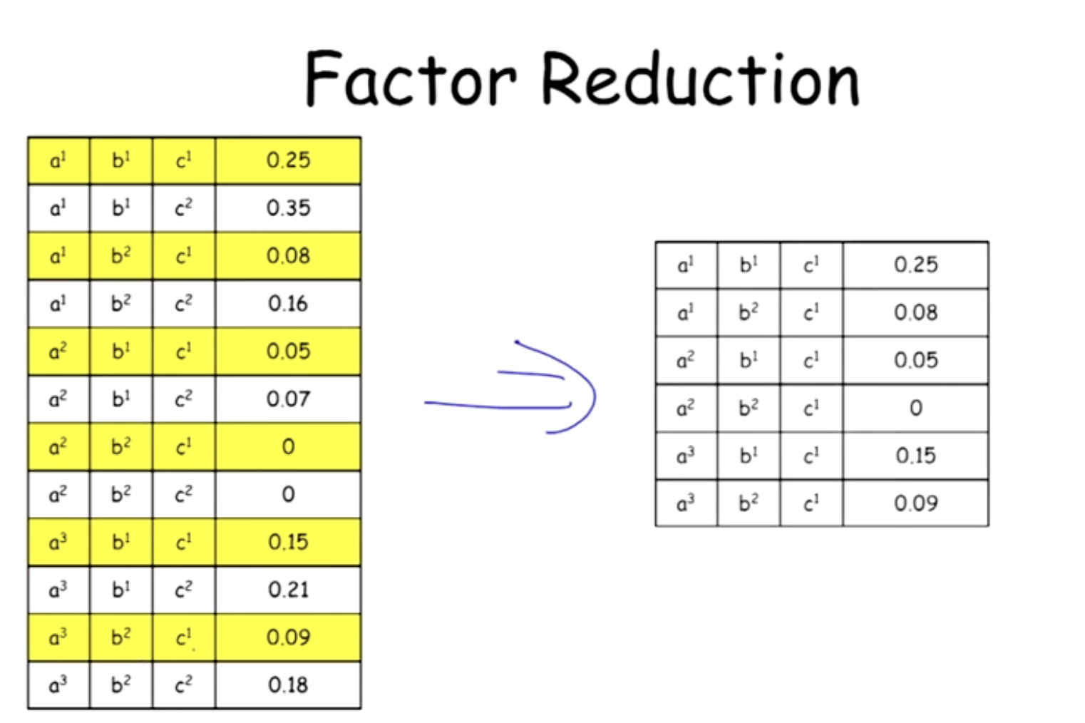
Factor Reduction(Conditioning)

3. Categories of PGM

2.1 Bayesian Network

The Bayesian Network use directed acyclic graph to represent the causally of random variables.

Each node \(X_i\) has a contional probability distribution(CPD) \(P(X_i|Par(X_i))\)

where par returns all parent nodes of \(Xi\) in the graph. If \(X_i\)does not has parent nodes, then replace the CPD with \(P(X_i)\)

A BN represent the JPD of all variables included, which can be calculated from: \[ P(X_1,X_2,...X_n) = \prod_i^n P(X_i|par(X_i)) \] We can say a joint probability P factorize over a graph G, if P can be represented by the above equation.

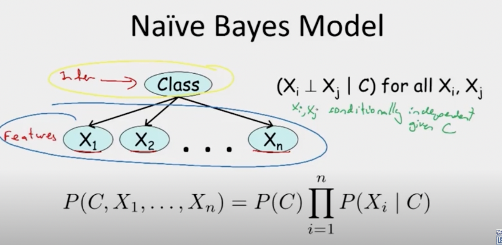
The Naive Bayes Model is an example of the simplistic BN. In naive bayes, assumptions are made that each feature are caused by a categorical variables, while the features remain independent to each other

2.2 Markov Random Field

2.2.1 Markov Chain and Transition Probability Matrix

Markov Chain

For a series of random variable \(X_1,X_2,..X_n\) we call this series a markov chain if: \[ P(X_m+1 = i_m+1| X_0=i_0,X_1=i_1,...X_m=i_m) = P(X_m+1 = i_m+1|X_m=i_m) \] In other word, the state of \(X_m+1\) depends only on the previous one state, which is the value of \(X_m\)

In many applications, we can use a markov chain to model the transition of states over time for a single random variable.

Transition Matrix

For any moment n, if the probability \(P(X_{n+1} = j|X_n =i)\) is independent to n, then we can this probability the one-step transition probability between state i and j, denoted as \(p_{i,j}\)

For all possible states of the random variable, the one-step probabilities between each two combinations consist the transition matrix. The sum of each row would be 1. Note that the sum of each column does not necessarily have to be 1.

2.2.2 Random Field and Clique

In a random field, each position(node) represent a random variable and can be assigned with a value.

In a graph, a clique is a subset of nodes that each two nodes in this subset are connected

If adding any nodes to a clique would no longer make that subset a clique, we call sucn a clique a maximal clique

2.2.3 Markov property of Random Field

Global Markov Assumption

For any two subsets of nodes S and T(S and T are not overlapped), given a separating subset C(a subset of nodes that all paths between S and T need to travel through this subset), if S and T are conditionally independent on C(\(P(S|T,C) = P(S| C)\))

Local Markov Assumption

Let V be any nodes in the graph, W be the adjacent nodes of V, O be other nodes in the graph. Given random variables \(X_W\), \(X_V\) and \(X_O\) are conditonally independent.

Pairwise Markov Assumption

Let U and V be two disconnected nodes in a graph, O be other nodes. Given random variables \(X_O\), \(X_U\) and \(X_V\) are conditionally independent

If any of the three assumption are satisfied in a random field, we call such a random field a Markov Random Field(MRF)

The Global Markov Assumption is the strongest one, the satisfaction of it implies the other two assumption

2.2.4 Potential Function of MRF

Potential Function

The potential function is defined on a clique in a MRF. It measure the correlation among the variables in the clique. the potenial function should be a non-negative function, and it should have greater value where one feels two variable correlated. For example, we can define a potential function that have maximum when to factors are equal.

Usually, we would define the potential function as a exponential function. \[ \phi_Q(X_Q) = e^{-H_Q(X_Q)} \] Where \(H_Q\) is called an energy function. The reason to adopt an exponential potential is that we can add the energy functions together when we multiply a potential function with another.

The usually format of a energy function: \[ H_Q(X_Q) = \sum_{u,v\in Q,u \ne v} \alpha_{u,v}t(x_u,x_v) + \sum_{v \in Q}\beta_{u,v}s(x_v) \] where:

• \(\alpha, \beta\) are hyper parameters
• t, s are functions to measure the energy between two nodes and asingle nodes. The could be just \(t(x_u,x_v) = x_ux_v, \ s(x_v)= x_v\)

Joint Probability

The joint probability a MRF represent can be calculated from a series of product of potential functions: \[ P(X_1,X_2,...X_n) = \frac{1}{Z} \prod_{Q \in C} \phi_Q(X_Q) \] Where Z is a scaling constant to ensure the probability is legal. In real application, the calculation of Z is very difficult because the number of cliques can be huge. We can instead calculate P based on maximal cliques: \[ P(X_1,X_2,...X_n) = \frac{1}{Z^*} \prod_{Q \in C^*} \phi_Q(X_Q) \] where \(C^*\) is the collections of all maximal clique in the MRF or subset of MRF