Sampling Methods for Machine Learning

Sampling and Simulation for Machine Learning

1. About Sampling and Simulation

The term "Sampling" can be used in different contexts in machine learning (ML). From a statistical perspective, sampling refers to the process of collecting a subset of units from a real sample population. The objective of sampling is to describe the characteristics of the sample through statistical analysis.

From a computational perspective, however, the term "Sampling" means "generating scenarios to represent a probability distribution" or in other words, "Simulation". In a computer context, "Sampling" actually refers to "Simulation". To clarify the distinction, in this article, sampling in a statistical context will be referred to as "Sampling", while sampling in a computational context will be referred to as "Simulation".

For Sampling

There are various sampling method that have each different application. Sampling methods can be categorized as:

1. Probability Sampling: Every Single unit in the population has a chance to be selected as a sample point
2. Non-Probability Sampling: Some units in the population does not have a chance to be selected as a sample point

From another dimension sampling methods can be categorized as:

1. Without Replacement : when a unit is selected, it would be taken out from the sample population
2. With Replacement: when a unit is selected, it would not be taken out from the sample population

This article focuses on sampling methods that has application in machine learning.

2. Sampling Method

2.1 Simple Random Sampling

In a random sampling, each unit in the sample population has a equal probability to be selected.

Pros:

• Easy to apply

Cons

• If the selection strategy is by any way associated with statistics through a confounder, a simpson paradox would be created
• If the researcher has any interests on the group differences among partition of the sample frame, SRS is not accommodate to it

2.2 Systematic Sampling

Systematic Sampling arranges all units in the population into some order, and then selecting elements at regular intervals through that ordered list.

Pros:

• It help avoid selection bias. The sample point are uniformly distributed on the section sorted by a particular order

Cons

• If there exists periodicity, and inner period of the order list is a multiple or factor of the interval we selected, the sample would be unrepresentative

2.3 Stratified Sampling

Stratified Sampling separates units into some "Strata" according to some categorical characteristics. The percentage of these strata is called a sampling fraction. A subsection of the sample is then assigned to each strata so that the proportion of each category of sample points is still the sample as sampling fraction. In each strata, sample are selected through SRS or systematic sampling.

Pros:

• It help avoid selection bias. The proportion of the category remains the same after sampling
• Researcher can apply different sampling method on different subgroup. This allow them to choose most suitable method for a subgroup

Cons

• Time-consuming and hard to design when a sample point has multiple characteristics

Stratified Sampling is the basic idea of many over-sampling and under sampling methods.

3. Monte Carlo Simulation

3.1 Inverse Transformation Sampling

We know that if a randam variable u = CDF(X), then u U(0,1) (refer to this article). The Inverse Transformation Sampling generate such a uniformly distributed random variab u U(0,1). Then the sample value X for each u would be

\[X = CDF^{-1}(u )\]

Pros: easy to apply

Cons: given P(X), CDF^{-1}(X) cannot always been easily obtained

3.2 MCMC Sampling

Markov Chain Monte Carlo (MCMC) sampling is a simulation technique used to approximate complex probability distributions. It is particularly useful when direct sampling from the distribution is difficult or infeasible.

MCMC sampling works by constructing a Markov chain that has the desired distribution as its stationary distribution. The chain explores the distribution by iteratively sampling from the current state and moving to a new state based on a set of transition probabilities. Through a large number of iterations, the chain converges to the desired distribution, allowing for efficient sampling.

MCMC sampling has various applications in machine learning, including Bayesian inference, parameter estimation, and model fitting. It is especially valuable when dealing with high-dimensional spaces or complex models.

Pros:

• Can sample from complex probability distributions
• Useful for Bayesian inference and model fitting

Cons:

• Can be computationally intensive
• Requires careful tuning of the Markov chain parameters

MCMC sampling is a powerful tool that enables researchers to explore and approximate complex probability distributions, making it an essential technique in machine learning and statistical modeling.

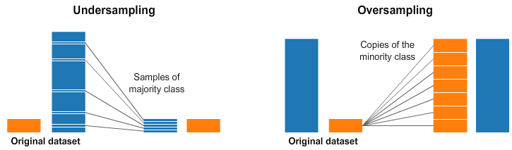
4. Resampling Methods for Imbalanced Data

An imbalanced dataset is one where the distribution of classes or categories is not equal or nearly equal. This can occur in various datasets, such as classification problems with multiple classes.

Imbalanced datasets pose challenges for machine learning algorithms as they can bias models towards the majority class, leading to poor performance in predicting the minority class. Addressing this issue requires specialized Resampling techniques.

A widely adopted technique for dealing with highly unbalanced datasets is called resampling. It consists of removing samples from the majority class (under-sampling) and / or adding more examples from the minority class (over-sampling).

4.1 Tomek Links

A Tomek Link exists between two samples if there are no other samples in their immediate vicinity.

Let \(x_i, x_j\) denote two sample points, \(d(x_i,x_j)\) denote the distance between these two points bu some measure, if:

1. \(x_i.x_j\) belong to different categories, and
2. There are no points \(x_k\) that satisfy \(d(x_k,x_i)<d(x_ i,x_j) \ or d(x_k,x_j)<d(x_ i,x_j)\)

then we call \((x_i,x_j)\) a tomek link. In other words, a Tomek Link represents a pair of samples that are the closest neighbors of each other, but belong to different classes. For a tomek link, there exists two possiblities:

1. at least one of \((x_i,x_j)\) is noisy
2. \((x_i,x_j)\) lies on the decision boundary

In either case, the classification model's performance would be undermined by the presence of tomek links. Therefore, we aim to eliminate the majority class instances involved in these links. This approach, known as under-sampling, is commonly used in imbalanced classification tasks. By removing the samples that form Tomek Links, we can better define the decision boundary between the majority and minority classes, which has the potential to improve the classifier's performance.

4.2 Edited Nearest Neighbors

Edited Nearest Neighbors (ENN) is an under-sampling technique used to reduce the number of samples in the majority class by removing instances that are misclassified by their nearest neighbors.

The ENN algorithm works as follows:

1. For each sample belongs to the majority class, find its k nearest neighbors based on a chosen distance metric.
2. If its class label differs from most of its neighbors, remove it from the dataset.

By iteratively applying this process, ENN aims to identify and remove noisy or misclassified instances from the majority class, thereby balancing the class distribution and potentially improving the performance of machine learning models.

ENN is a relatively simple and effective method for under-sampling in imbalanced datasets. However, it is important to note that ENN may discard informative instances if they happen to be misclassified by their nearest neighbors. Thus, the choice of the number of nearest neighbors (k) and the distance metric should be carefully considered to achieve the desired balance between class distribution and information preservation. Besides, as the number of minority points is relatively fewer, the points we can discard by ENN is limited.

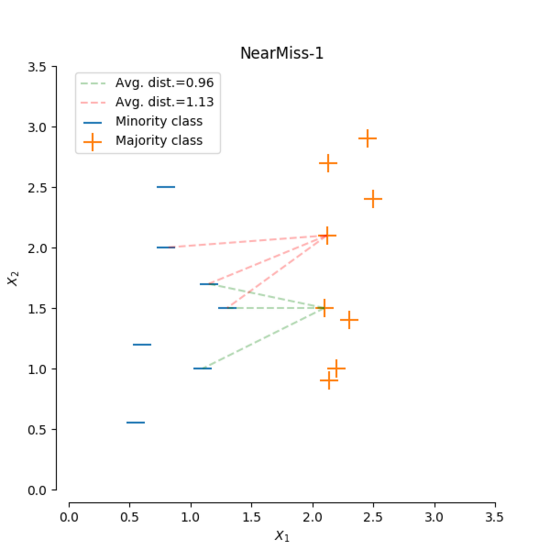
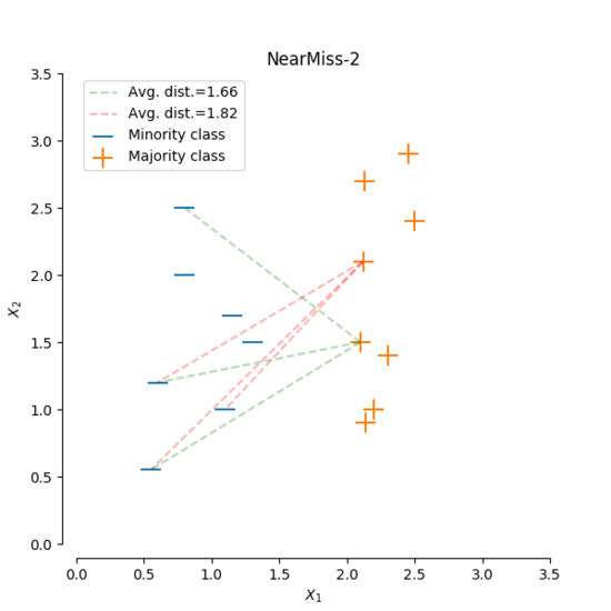
4.3 NearMiss

NearMiss is an under-sampling technique commonly used for imbalanced datasets. It aims to select a subset of samples from the majority class that are "near" to the minority class.

There are three variations of the NearMiss algorithm:

1. NearMiss-1: Reserve samples from the majority class that have the smallest average distance to the k nearest neighbors in the minority class.
2. NearMiss-2: Reserve samples from the majority class that have the farthest average distance to the k nearest neighbors in the minority class.
3. NearMiss-3: Selects samples from the minority class and reserve the k nearest neighbors of it in the majority class

The NearMiss algorithm helps to address class imbalance by reducing the dominance of the majority class. By selecting samples that are "near" to the minority class, it aims to improve the classification performance on the minority class.

It is important to note that the choice of the NearMiss variant depends on the specific dataset and problem at hand.

An advantage of NearMiss is that the number(or the ration of number) of samples in majority class is controllable

4.4 Ensemble Methods

Except for specific algorithms, there are also some approaches based on ensemble learning that can be used to perform undersampling.

EasyEnsemble

EasyEnsemble is an ensemble learning technique specifically designed for imbalanced classification tasks. It works by creating multiple subsets of the majority class and combining them with the entire minority class. Each subset is created by randomly under-sampling (with replacement) the majority class to balance its distribution, or we can say, number, with the minority class. The resulting subsets are then used to train individual models.

During prediction, each model in the ensemble is used to make predictions, and the final prediction is determined by aggregating the predictions of all models. This approach helps to improve the classification performance on the minority class by giving more weight to its predictions.

It is worth noting that the number of subsets created in EasyEnsemble can be adjusted based on the severity of class imbalance and the available computational resources. The more subsets created, the more emphasis is placed on balancing the class distribution.

BalanceCascade

BalanceCascade is an ensemble learning technique commonly used for imbalanced classification tasks. It is an extension of the EasyEnsemble method and aims to further improve the classification performance on the minority class.

BalanceCascade works by iteratively training and combining multiple models. We train the model with the current dataset and obtain the classification results. Then, the misclassified instances from the majority class in the current dataset are identified and removed. This process is repeated for a predefined number of iterations or until a stopping criterion is met.

By iteratively focusing on the misclassified instances of the majority class, BalanceCascade aims to improve the classification performance by gradually reducing the impact of the majority class on the final prediction. This iterative process helps to refine the decision boundary between the classes and enhance the model's ability to correctly classify the minority class.

4.5 Synthetic Minority Oversampling Technique(SMOTE)

SMOTE

The Synthetic Minority Oversampling Technique (SMOTE) is a popular algorithm used for oversampling in imbalanced classification tasks. SMOTE works by creating synthetic examples of the minority class to balance the class distribution.

The SMOTE algorithm can be summarized in the following steps:

1. For a sample \(x_i\) in the minority class, find its k nearest neighbors, denoted as \(NN\)

2. Randomly select(with replacement) \(x_{nn} \in NN\), make an interpolation by \[ x_s = x_i + (x_{nn} - x_i) * rand(0, 1) \] where \(rand(0,1)\) is a random number between 0 and 1, add \(x_s\) to the minority class dataset.

3. Repeat steps 1 and 2 until the desired level of oversampling is achieved.

By generating synthetic examples, SMOTE effectively increases the representation of the minority class in the dataset.

It is important to note that the choice of the number of nearest neighbors \(k\) in SMOTE and the distance metric can affect the quality of the synthetic examples and the performance of the resulting models.

Additionally, there’s a trade-off for SMOTE. On one hand, if the selected minority class samples are surrounded by majority class samples, this minority sample points can be an invading noisy point or a point lies near the decision boundary. As a result, the newly synthesized samples will overlap significantly with the surrounding majority class samples, which is called an invasion, leading to classification difficulties. On the other hand, if the selected minority class samples are surrounded by other minority class samples, the newly synthesized samples will not provide much useful information, as it is far from the decision boundary(which is also a noisy point to some degree).

The former situation can be solved by append under-sampling method, such as Tomek links, right after the SMOTE algorithm. For the later situation, we can introduce Borderline-SMOTE

Borderline-SMOTE

Borderline-SMOTE is an enhanced version of SMOTE that focuses on generating synthetic examples near the decision boundary between the minority and majority classes.

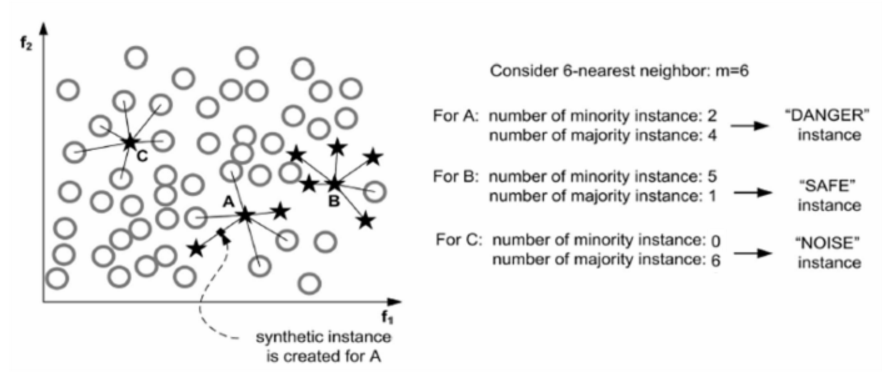
Let \(S\) denote the collection of minority sample points, \(L\) denote the collection of majority sample points, \(T\) denote the collection of all sample points. The Borderline-SMOTE algorithm can be summarized in the following steps:

1. For \(s\) in \(S\) , find the k nearest neighbors, denoted as \(NN\) , let \(m\) denote the number of points in \(NN\) that belongs to \(L\) : \(m = |NN \cap L|\)
2. Classify \(s\) according to \(m\)
   1. If \(m = k\), then \(s\) is noise(invasion)
   2. if \(\frac{k}{2}\le m <k\), then \(s\) is danger(near decision boundary)
   3. if \(0\le m <\frac{k}{2}\), then \(s\) is safe(lack of information)
3. Only when \(s\) is danger, implement SMOTE on \(s\) and generate synthetic examples
4. Repeat step 1-3 for next point in \(S\)

By generating synthetic examples near the decision boundary, Borderline-SMOTE aims to improve the classification performance on the minority class while avoiding the creation of invasion samples or noisy samples in regions far from the decision boundary.

The algorithm above is in some cases called Borderline-SMOTE 1, as there is another version called Borderline-SMOTE 2. The difference between these two versions is in step 3. For Borderline-SMOTE 2, the step 3 is:

1. Only when \(s\) is danger:
   1. respectively find its k nearest neighbors in \(L\) and \(S\) , denoted as \(NN_L\) and \(NN_S\) , let \(n\) denote the total number of synthetic samples we want to generate
   2. Generate \(\alpha n\) points with SMOTE on samples in \(NN_S\)
   3. Generate \((1-\alpha) n\) points with SMOTE on samples in \(NN_L\)

where \(\alpha\) is a parameter controlling the ratio of synthetic samples we generate along the two sides of the decision boundary. This can control the invasions to some extent.

4.6 ADASYN

ADASYN (Adaptive Synthetic Sampling) is an oversampling technique designed to address the class imbalance problem in imbalanced datasets. It focuses on generating synthetic examples according the distribution of the minority class data points.

The ADASYN algorithm can be summarized in the following steps:

1. Calculate the class imbalance ratio, which is the ratio of the number of majority class samples to the number of minority class samples: \(d = \frac{n_S}{n_L}\)
2. If \(d\) is smaller than a preset threshold, than the dataset is imbalanced enough, otherwise, end the algorithm
3. Calculate the number of synthetic examples to generate for \(G\):

\[ G = (n_L - n_S)\beta \]

where \(\beta\) is a controlling parameter . When \(\beta = 1\), the number of samples from the minority class will be supplemented to match the number of samples from the majority class.

4. For each point \(x_i\) in \(S\) , identify the k nearest neighbors of the \(s\) , denoted as \(NN\), let \(r_i\) denote the ratio of points in \(NN\) that belongs to the majority class:

\[ r_i = \frac{|NN \cap L |}{|NN|} \]

5. For each point \(x_i\) in \(S\), compute the density of it: \[ p_i = \frac{r_i}{\sum_ i^{n_s}r_i} \]

6. For each point \(x_i\) in \(S\), generate \(p_i *G\) synthetic samples with SMOTE

ADASYN adapts the synthetic generation process based on the local density distribution of the minority class. It generates more synthetic examples for samples that are in regions with a lower density of minority class samples, making the synthetic examples more informative and challenging for classification.

A problem of ADASYN is that it may cause invasion, as it can generate more samples near invading noisy point. We can introduce other methods, such as borderline SMOTE or Tomek links to solve this problem.