Structural Causal Model

Introduction of Structual Causal Model

1. About Structural Causal Model

The Structural Causal Model(SCM) is another framework of causal inference. It is a way of describing the relevant features of the world and how they interact with each other. It is widely used in causal relationship digging.

2. Basis of Graph Theory

Graph: a collection of vertices(nodes) and edges. The nodes are connected by edges.

Adjacent: If there is a edge between two nodes, then these two nodes are adjacent

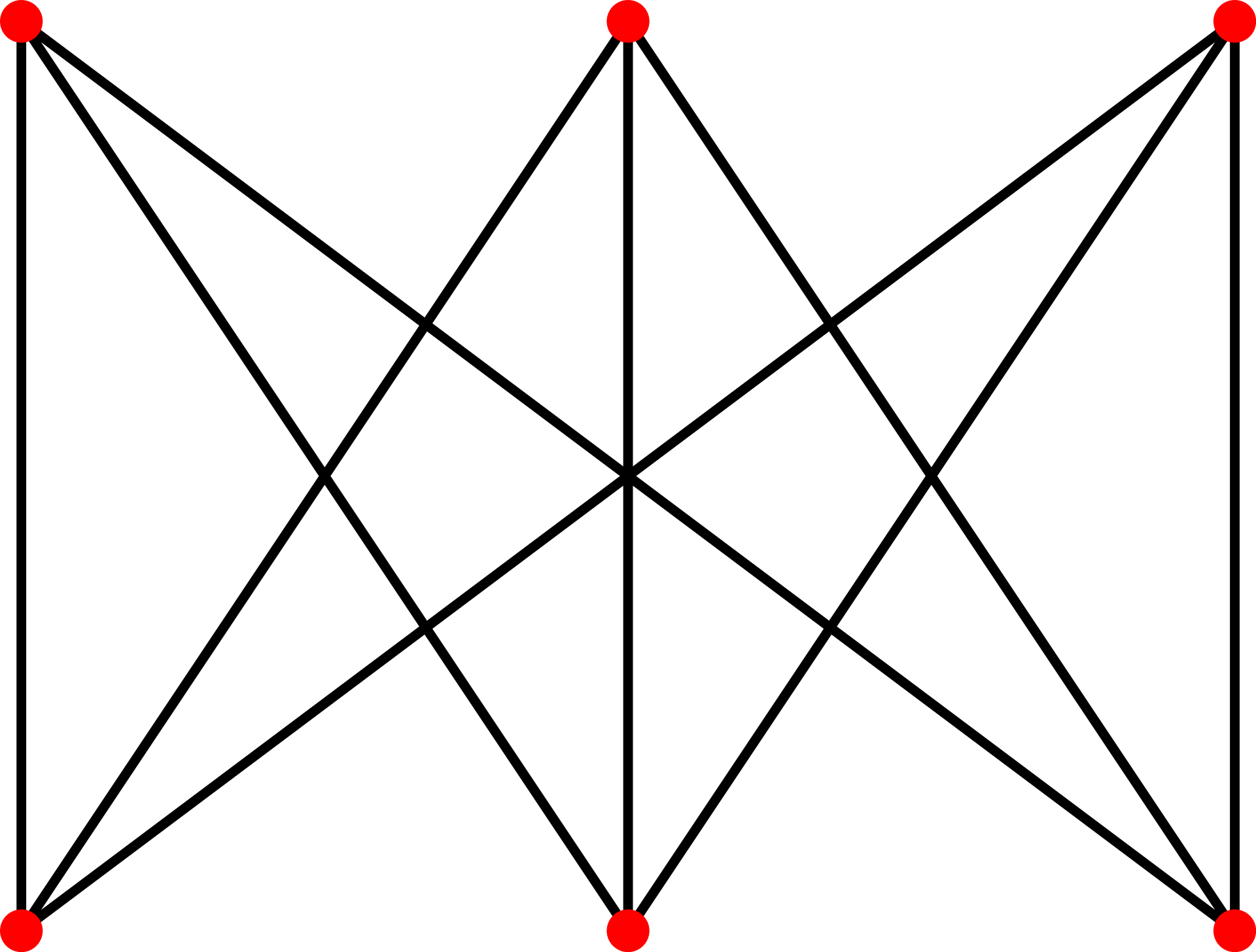
Compete Graph: A graph is a complete graph if every pair of nodes in it is adjacent

Path: A sequence of adjacent nodes and their edges between node X and node Y is called a path between X and Y

Directed/Undirected Graph: An edge can be directedor undirected. If all edges in a graph is directed, this graph is a directed graph

Directed Path: If every edges in a path have same directions, then this path is a directed path

Parent/Child: The Start and End nodes of the directed graph

Ancestor/Descendant: For a directed path,the ancestor nodes are all nodes before this node, the descendant nodes are all nodes after that node

Cyclic: when a directed graph contains a path that its starting node and ending node are the same node, then this path is called a cyclic

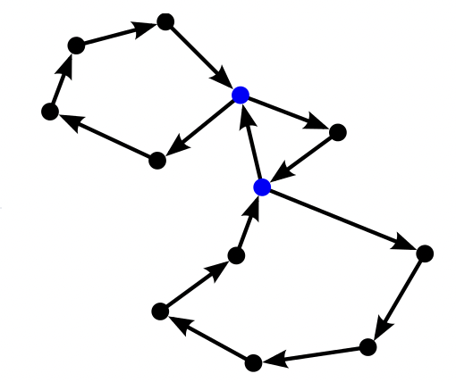
DAG: A directed graph with no cyclics in it is called a Directed Acyclic Graph(DAG)

3. Basic Theory of SCM

3.1 Causility

In SCM, the causality is considered as function with a time order. For two variable X and Y, we call X a direct cause of Y if: \[ Y = f(X) \] note that there's a time order for the happenings of X and Y. We cannot regard the cause as \(X= f^{-1}(Y)\)

We call X a indirect cause of Y is X is a cause of any cause(direct or indirect) of Y.

In SCM, the relationship of a direct cause X, an outcome Y and their causality f is presented with a parent node. a child node and the directed edge between them.

In most case, a causility would demonstrate statistical dependence on observations. From a probability aspect, we can also interpret this correlation as a joint probability. For an causal graph: \[ P(X_1,X_2,...X_n) = \prod_i^n P(X_i|par(X_i)) \] where \(par(X_i)\) is all parent nodes of \(X_i\). If \(X_i\) does not have a parent node(Exogenous), then just apply\(P(X_i)\)

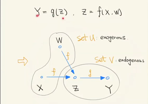
3.2 Exogenous/Endogenous Variable

In SCM, the exogenous variables, usually denoted as U, are variables considered external to the model, and we would not explained how these variables are caused. Oppositely, the endogenous variable,usually denoted as V, are variables considered a descendant of at least one exogenous variable. Exogenous variables have no ancestors, only descendants, while endogenous variables have both ancestors and descendants.

With such assumption, we can represent the causality of variables with a DAG.

In a causality DAG, only when there's a directed path between two variables can we regard as there exists a direct or indirect causality between these two variable.

3.3 Intransitive Case

As discussed in this article, we know that correlation does not imply causality. On the opposite, if X causes Y, then in most case X and Y are statistically dependent. Nevertheless, there still exists some extreme case where causality does not show statistical correlation.

For example, suppose gene A can increase a person's risk of getting a cancer, while there exists another gene B that can depress people's risk of getting cancer. If we observe a sample where each person has both gene A and B, we probably would get the conclusion that both gene are independent to the rate of getting a cancer.

Another example is the "exclusive or" logic, if the two inputs are both binary variable with equal probability, and the output is a EO calculation of the two binary example, then the output are independent to each of the two inputs from a probability perspective.

Other cases might be found in real application, we cannot always expect that causality would always generate statistical significant difference. However, we still believe in most cases the significance would be showned, which is the basic assumption for causal inference

3.4 Basic Structure for Causality Graph

3.4.1 Chain, Fork and Colider

The basic causal structure in SCM can be concluded into three types, and each type describes the relationship among three Causal Structure in SCM

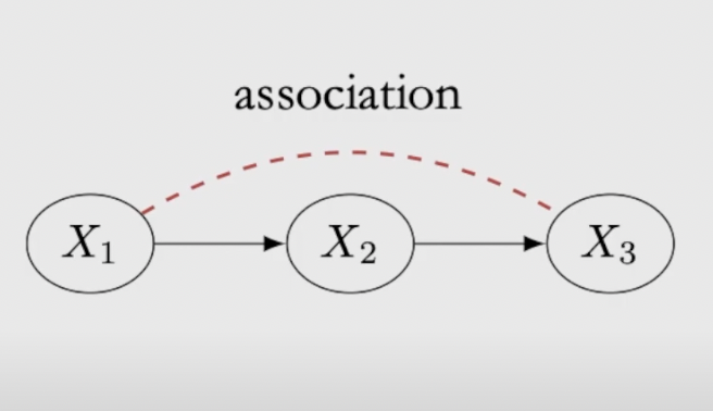
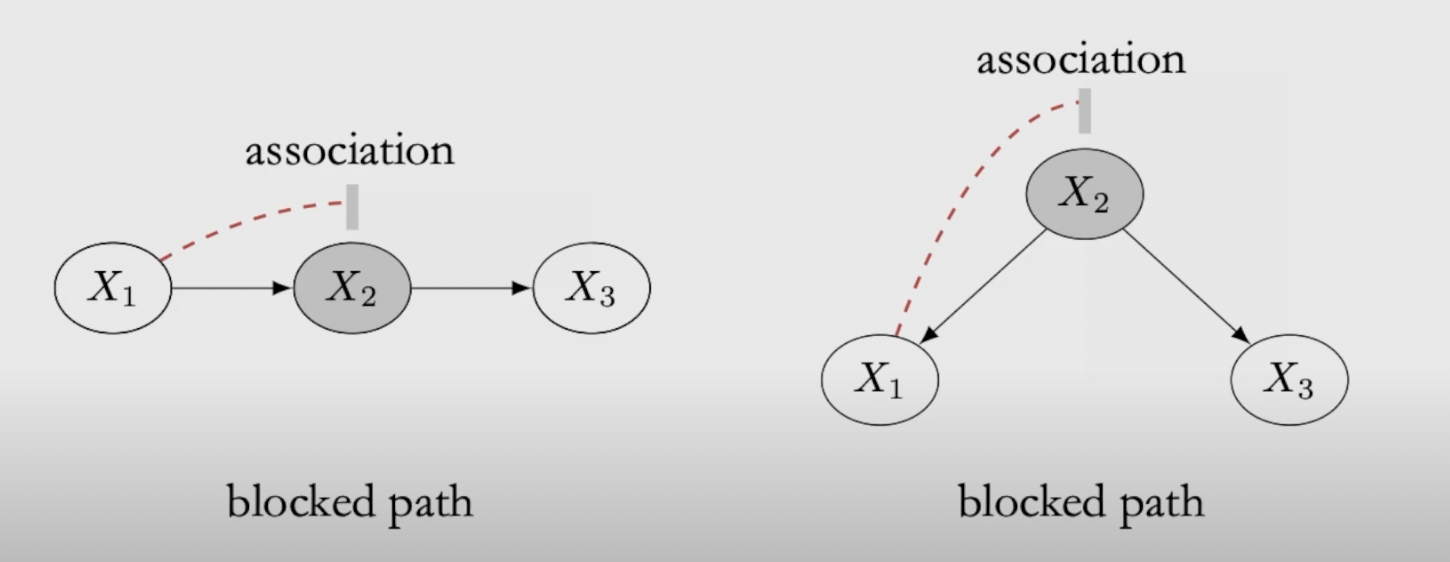
Chain: For a chain, the first node and the last node are statistically depent, association flows through the directed path, to block the association, we need to conditioning on \(X_ 2\)

Fork: For a fork, the two descendant nodes are statistically depent, association flows through the path even if its indirected, to block the association, we need to conditioning on \(X_ 2\)

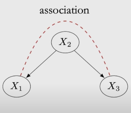
Colider : For a colider, the two parent nodes are not statistically depent, the intermediate nodes naturally block the association without conditioning

Conditioning : conditioning means segment samples into subgroups according to certain values. In a SCM context, if we condition the intermediate variable, we can regard it as a constant in causality:

• For a chain, before conditioning, \(X_3 = f(X_2,u_3) = f(g(X_1),u_3)\), after conditioning, \(X_3 = f(u_3)\)
• For a fork, before conditioning, \(X_3 = f(X_2,u_3), X_1 = f(X_2,u_1)\), after conditioning, \(X_3 = f(u_3), X_1 = f(u_1)\)
• For a colider, before conditioning, \(X_1 = f(u_1),X_ 3=f(u_ 3)\), after conditioning on \(X_2\) or any of its descendants, although the cause of \(X_1\) and \(X_3\) remains the same, we now have \(X_ 2 = f(X_1,X_3) = c\), so statistical dependence would appear between \(X_1\) and \(X_3\)

3.4.2 D-separate

D-separation is a method used to determine whether two nodes in a causal graph is statistically independent.

• \(X \ and \ Y \ are \ d-sep \iff X \ and \ Y \ are \ statistically \ indepentdent\)
• $X  d-sep  Y | Z X  and  Y  are  statistically  indepentdent | Z $

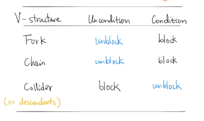
From the previous section we know that in a V structure,

1. If the cenral node are not conditioned, two nodes are blockd by a colider and unblocked(d-connected) by a chain or a fork.
2. If the cenral node are conditioned, two nodes are blockd by a chain or a fork and unblocked by a colider.

If every paths between two nodes X and Y are blocked, we called X and Y d-separated.

4. Causality Search

4.1 Test on Causality Model

With the definition of the D-separation, we can test the causal model we assume by examine where the statistical independence inferred from the model can be validated through data. For example, for such a causal model:

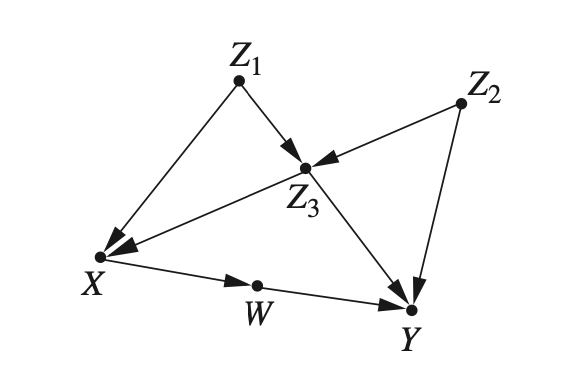
The path \(W \to X \to Z_1\) should be blocked if we conditioned on X, which means this model implies: \(Z_1 \perp \!\!\! \perp W\ |X\)

We can then regress a linaer model \(Z_1 = r_1W + r_2X\), if \(r_ 1\) is obviously greater than 0, we can regard as the assumed causal model is incorrect. We can also apply other statistical method to test correlation.

Through this kind of ideas, we can infer the true causal model by testing potential causal models based on dataset

4.2 Equivalent Class

For some causal relationship, we may found two different potential causal graph of it appears to have same statistical independent on data. For example, a fork and a chain have same relationship on statistical independence. When we try to infer the causal relationship, we might found some causility, or we can say the directions of some edgs in the DAG, cannot be decided through data. In this case, we call these potential models with same statistical independence appearance Equivalent Classes

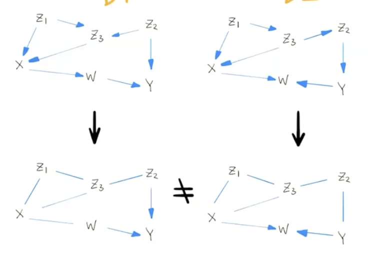
A intuitive method to judge whether two graph are equivalent classes is to check each V-structure in for both graph and earse the direction of the edges if the two V-struture are equivalent. If there are no directions left, then the two classes are equivalent. If there are remaining directed edges or V-structure that are different, then the two graphs are not equivalent.

5. Causal Discovery Algorithm

The basic problem of Structual Causal Learning is:

1. Structure Learning: Causal Discovey. To find out the causal relationship among variables and depict it as a probability graph
2. Parameter Estimation: When the causal structure is found, find the parameter of conditional probability distribution so that we can apply bayesian chain rule.

For Parameter Estimation, refer to this blog. For Causal Discovery, the algorithm to implement includes three types:

• Constraint-based Algorithms: This class of algorithms learn a set of causal graphs which satisfy the conditional independence embedded in the data. These algorithms use statistical tests to verify if a candidate graph fits all the independence based on the faithfulness assumption. Examples are PC algorithm, FCI, and GFCI
• Score-based Algorithms: This type of algorithm replaces conditional independence tests with the goodness of fit tests. Score-based algorithms learn causal graphs by maximizing the scoring criterion which returns the score of the causal graph given data. Examples are Greedy Equivalence Search (GES)、FGES
• Algorithms based on Functional Causal Models (FCMs): In FCMs, a variable can be written as a function of its directed causes and some noise term. Examples are Linear Non-Gaussian Acyclic Model (LiNGAM)、ICA-LiNGAM