Potential Outcome Framework

Introduction of Potential Outcome Framework

1. Potential Outcomes Framework

The Potential Outcomes framework is a series of notation widely used in causal inference.

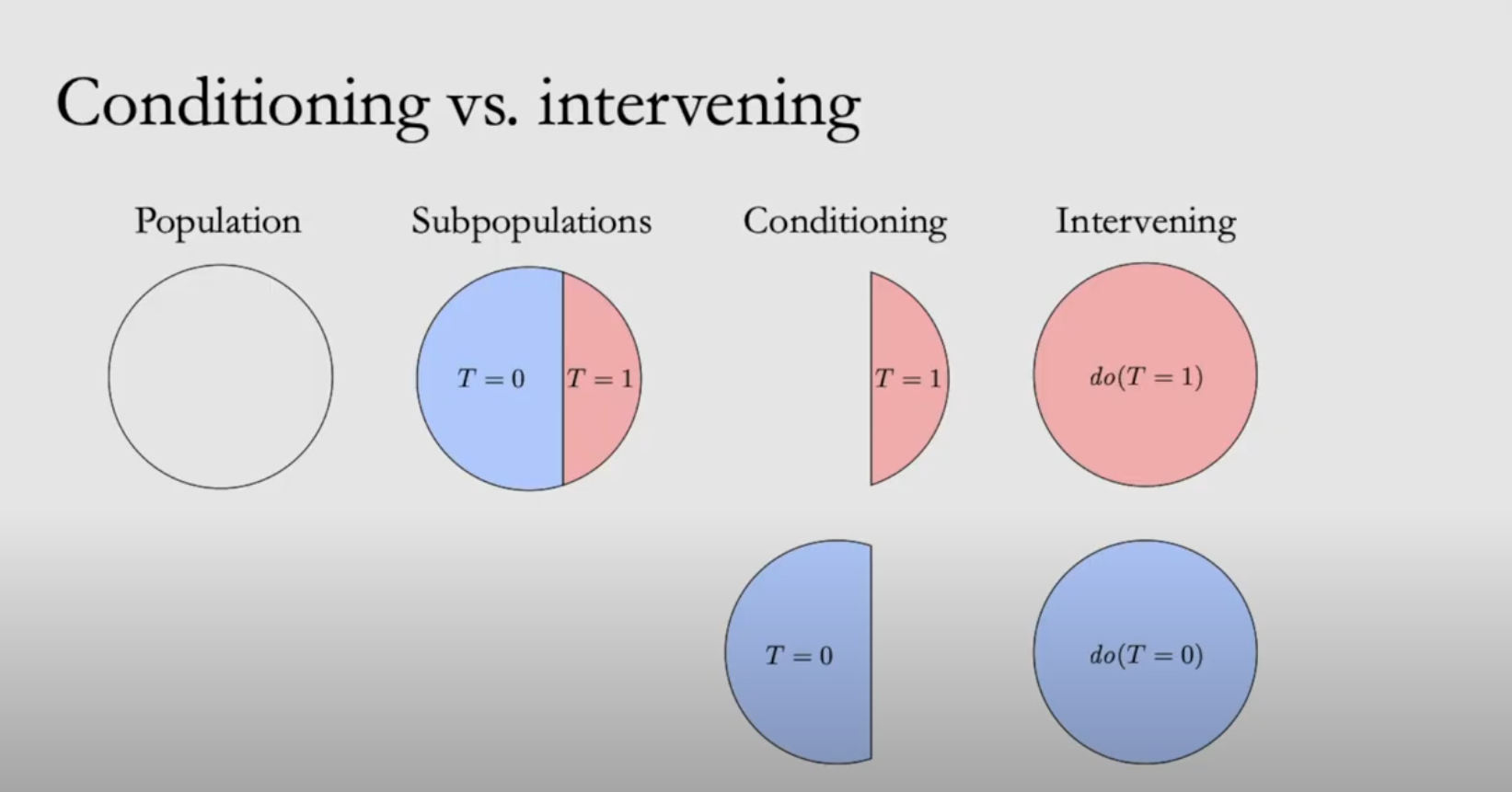
1.1 Conditioning v.s. Intervening

In statistics, conditioning and intervening is two different concepts.

Conditioning: Segmenting a dataset into subset bu applying conditions on variables

Intervening: Intervene a process with certain treatment, so that every unit is affected by treatment variable

we use the do operands the represent that we intervene a process. It forces T to be the value we want, and thus makes T independent to any confounders X. Let Y donate the outcome statistics of the process, the probability of Y = y under a intervention such that T=t is noted as \(P(Y=y|do(T=t))\) or \(P(y|do(t))\)

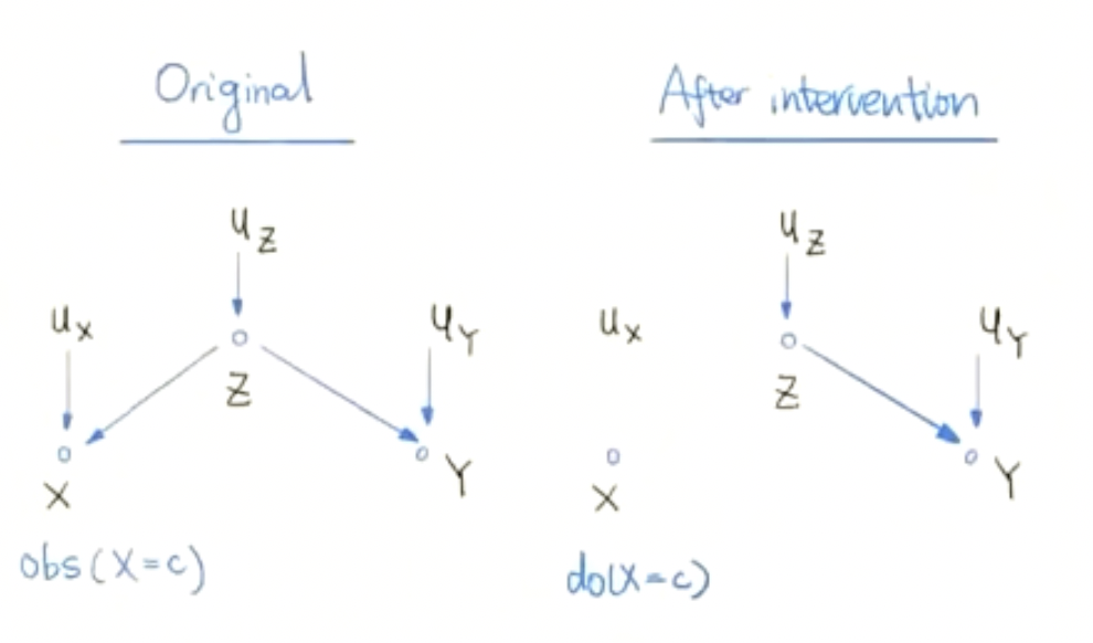
When there exists confounder in the process, the conditional probability does not equal the interventional probability: \[ P (Y|do(t),X) = E_X[P(Y|T=t,X)] \ne P(Y|T=t,X) \]

1.2 Potential Outcomes

Suppose we want to evaluate the cause effect of a pill on a single person.

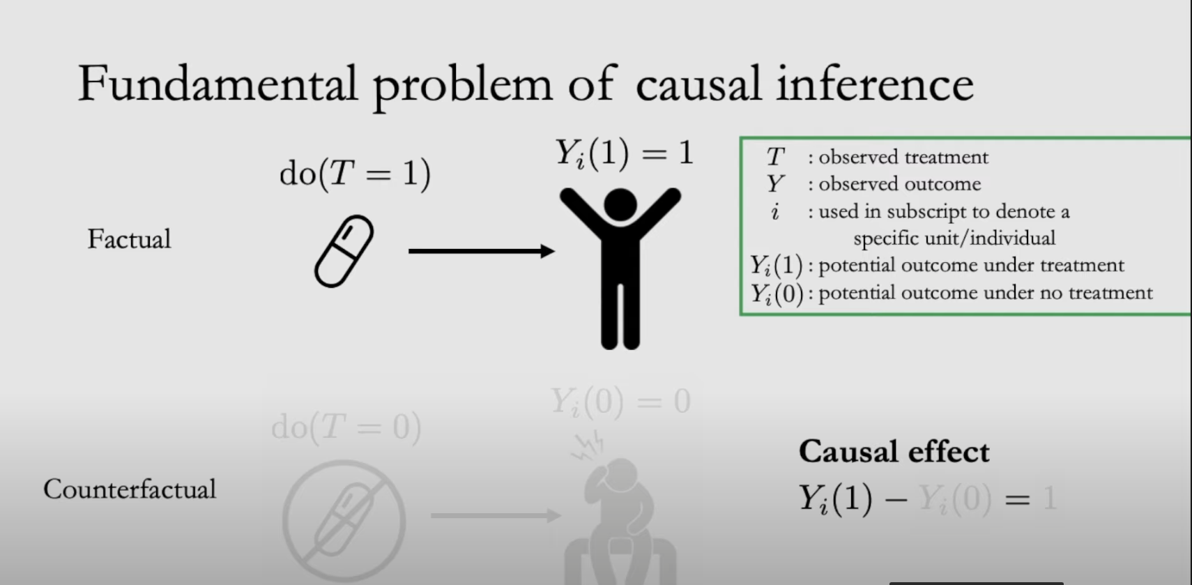
Let T denotes whether this person take a pill, Y denotes the degree that his headache is relieved after taking the pill. The Cause Effect can be noted as: \[ Y|do(T=1) \ - Y|do( T =0) = Y(1)-Y(0) \] The cause effect of a treatment on a single unit is called Individual Treatment Effect(ITE)

A problem of evaluating the effect this way is that for a single person we can only observe Y for once. If we intervene the treatment so that T = 1, we won't obtain any observations about Y(0).

In such case, we call Y(1),Y(0) the potential outcomes under T. A potential outcome is the outcome of the statistics under our potential treatment.

For a specific unit, suppose we applied treatment T=t on it, we call the observed outcome \(Y^F= Y(T=t)\) the factual outcome. The potential outcome that not applying T=t, \(Y^{CF} = Y(T\ne t)\) is called the counterfactual outcome. \(Y^{CF }(T =1) = Y^F(T=0)\)

1.3 Basic Assumptions about Potential Outcomes

Stable Unit Treatment Value Assumption(SUTVA): The potential outcome of any unit won't be changed by treatment on other units. This assumption emphasize the independency of units

Positivity Assumption: For units of any possible values of background variable, any assigned treatment is possible. \[ P(T=t|X=x) \in (0,1) \quad \forall t\ and \ x \] Consistency Assumption : If T=t is applied on a group of unit, then the outcomes of all units in that group would be Y(T=t). \[ T = t \Rightarrow Y=Y(t) \] The consistency assumption make sure we have $Y(t) = Y|T=t $ when there's no confounders

Ignorability Assumption: The determination of the treatment T is independent to the potential outcomes: \[ (Y(1),Y(0)) \perp \!\!\! \perp T \] Under the Ignorability Assumption: \[ E[Y(1)] = E[Y(1)|T=1] = E[Y| T=1] \] The Ignorability Assumption is also called unconfoundedness assumption . It indicates there are no confounders taking effects in the causality. Ignorability Assumption is usually considered satisfied when we conduct a random control trail. If we randomized the determination of the treatment, the treatment delivered to a single unit is decided only by randomness, not any confounders. This implies the influence of the confounders are blocked. However, in a non-experimental context, since T is not randomized, the influence of the confounder still exists, and the Ignorability Assumption is not satisfied.

Conditional Ignorability Assumption: Given background variables X, the determination of the treatment T is independent to the potential outcomes \[ (Y(1),Y(0)) \perp \!\!\! \perp T \qquad |X \] Under the conditional Conditional Ignorability Assumption: \[ E[Y(1)|X=x_i] = E[Y(1)|T=1,X=x_i] = E[Y| T=1,X=x_i] \] The Conditional Ignorability Assumption is also called no unmeasured confounders assumption. It means all confounders are detected and we can thus estimate causal effect through conditioning on X. There's no potential confounders unmeasured.

With these assumption, we can make the following statement for a causal inference process:

• The SUTVA, Positivity and Consistency should always be satisfied

• If a RCT is conducted, we can regard as \((Y(1),Y(0)) \perp \!\!\! \perp T\), and The ignorability assumption can be considered satisfied. Thus a RCT is a best solution for causal inference

• If RCT is not implementable, we can condition on the confounder to satisfy the conditional ignorability assumption and estimate the CATE, then we may estimate the distribution of the confounders and calculate the exception of the CATE to obtain ATE

  

1.4 Average Treatment Effect

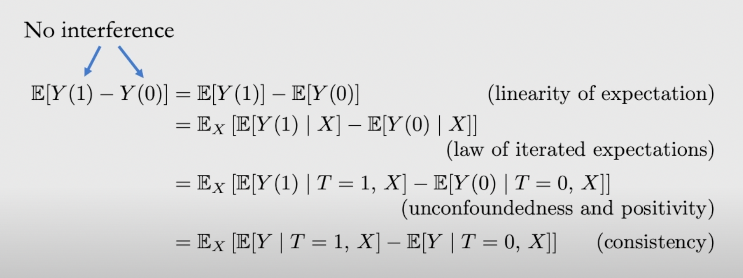
Due to the problem discussed in 1.2, we usually cannot get the ITE of a treatment directly. However, if we do not put specific emphasis on the effect of individual, we can obtain the overall effect size by calculating the Average Treatment Effect(ATE) of a treatment on a population: \[ ATE = E[ITE] =E[Y^F(T=1)] - E[Y^{CF}(T=1)] = E[Y(1)] - E[Y(0)] \] When the ignorability assumption is fulfilled, there exists no confounders: \[ E[Y(1)] = E[Y|T=1] \]

When the Ignorability Assumption is not fulfilled, but the conditional ignorability assumption \[ E[Y(1)] = E_x[E[Y( 1)|X=x]=E_X[E[Y|T=1,X=x]] \] here the X follows its original distribution \(X \sim D(\theta)\)

However, when we try to interpret the effect size from observational data, what we actually obtained is \[ E[Y|T=1] - E[Y|T=0] = E_{X_T}[E[Y|T=1,X_1]] - E_{X_C}[E[Y|T=0,X_0]] \] Here \(X_T\) and \(X_C\) follow conditional probability distributions given T instead of X's original distribution: \(X_1 = (X| T =1), X_0 = (X|T=0)\), \(X_1 \sim D(\theta_1), X_0 \sim D(\theta_0)\)

when confounder exists, X would have different distribution on the treatment and control group, thus \[ P(X_T) \ne^d P(X_C) \] Thus, when confounder exists: \[ \begin{aligned} E[Y(1) - Y(0)] & \ne E[Y|T=1] - E[Y|T=0]\\ E[Y(1) - Y(0)] &= E_X[E[(Y|T=1,X)] - E[(Y|T=0,X)]]\\ &= \sum_ x(E[Y|X,T=1]-E[Y|X,T=0])P(X) \end{aligned} \]

This is called the adjustment formulation in causal inference. To obtain the causal effect, we need to condition on \(X\), obtain CATE, estimate the distribution of X and finally compute ATE. This can be unrealistic since in many occasions \(X\) can be really high-dimensional. To solve this problem, various type of causal inference methods are proposed.

1.5 CATE, ATT and ATC

Conditional Average Treatment Effect

Conditional Average Treatment Effect (CATE) is the average treatment effect (ATE) for a subset of the population that satisfy certain conditions. Under Conditional Ignorability Assumption: \[ CATE(x_ i) = E[ Y(1)-Y(0)|X=x_i] = E[Y|T= 1,X=x_i]- E[Y|T= 0,X=x_i] \] In most real application cases, there are multiple confounders in the causal inference process. To estimate the ATE, we need to "block" the effects of confounder. We calculate the weighted average of the CATE as the ATE estimation. The weight is the probability of the segmentation in the whole population. Such kind of methods are called Backdoor Adjustment: \[ ATE = E_X[CATE(x_ i)] = E_X[E[Y|T=1,X= x_i]- E[Y|T=0,X= x_i]] \] Average Treatment Effect on Treated(ATT)

ATT is an econometric concept used to measure the causal impact, in other word, the average difference between potential outcomes of a treatment or intervention on a specific subgroup within a population, namely those who actually received the treatment. \[ ATT = E[Y(1)|T=1] - E[Y(0)|T=1] \] When \(T\) is fixed as 1, we know that the distribution of confounders \(X\) is fixed as \(P(X|T= 1)\). Thus: \[ \begin{aligned} ATT & = E[Y(1)-Y(0)|T=1]\\ & = E_{X|T=1}[E[Y|X,T=1]-E[Y|X,T=0]|T=1]\\ &= E_{X|T=1}[E[Y|X,T=1]-E[Y|X,T=0]] \qquad Conditional\ Ignorability \\ &= \sum_x (E[Y|X,T=1]-E[Y|X,T=0]) * P(X|T=1) \end{aligned} \] We can samely obtained the Average Treatment Effect on Controlled(ATC) as: \[ ATC = \sum_x (E[Y|T=1]-E[Y|T=0]) * P(X=x|T=0) \]