Introduction of Causal Inference

1. About Causal Inference

Causal Inference refer to the process that we want to discover the real causality between variables based on data. Specifically, there are two domains of causal inference:

• Causality Discovery: find the causal structure among variables
• Causal Effect Estimation: give a quantitative evaluation on the causal effect of a variable to another

2. Why Causal Inference

The core reason why we cannot discover causal realtionship and estimate causal effect through traditional statistical methods is that: Correlation does not imply Causality. Use traditional Statistics methodology, which is basically based on statistical dependence, on causal reasoning would lead to bias

2.1 Simpson Paradox: Confounder

Suppose we have two treatment A and B for a certain disease and want to evaluate if A has better effect by cure rate. There are two categories pf patients: mild patients and severe patients. Suppose the truth is condition of patients have effects on both the selection of treatment and the cure rate:

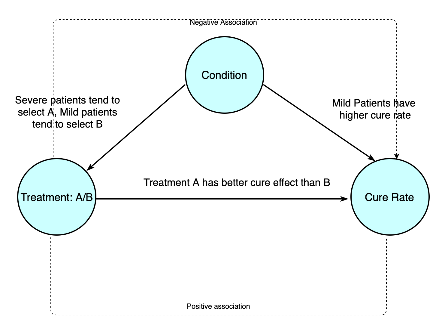
However, since we failded to recognize the ture causal relationship among these variables, we assume there's no other facor other than treatment and effect:

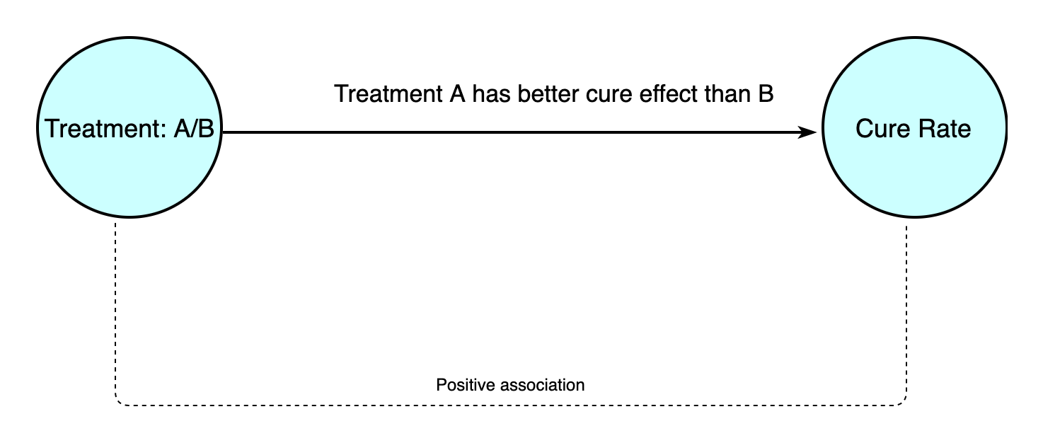
Under these assumption, we obtained the following data:

Treatment	Mild	Severe	Total
A	\(\frac{30}{100} = 30\%\)	\(\frac{210}{1400} = 15\%\)	\(\frac{240}{100} = 16\%\)
B	\(\frac{100}{500} = 20\%\)	\(\frac{5}{50} = 10\%\)	\(\frac{105}{550} = 19\%\)

Here a simpson paradox appears: treatment A is better than treatment B on every segments, but the overall effect of A is actually lower.

The occurrence of simpson paradox usually suggest the existence of confounder variables. If one or more variables have causal effects on both of two variable, we call these variables confounders of the two variables. In this case, the condition is a confounder.

Let Y denote the cure rate, X denote the condition of patients, and T denote the selection of treatment. For these data, what we observed is: \[ E[Y|T= A] - E[Y| T= B] = 16\%-19\% = -3\% \] under the wrong assumption that there's no confounding variables, we believe: \[ E[Y(A) - Y(B)] =E[(Y|T=A) - (Y|T=B)] = E[Y|T= A] - E[Y| T= B] = -3\% \] and we draw the conclusion that A has negative effect.

However, the truth is, the when there are confounders, the true interpretation of the results ought to be: \[ E[Y(A) - Y(B)] = E_x[E[(Y|T=A,C) - (Y|T=B,C)]] = \sum_i P(C=i)E[(Y|T=A,C) - (Y|T=B,C)] \]

\[ E[Y(A) - Y(B)] = \frac{600}{2050}*(0.3-0.2)+\frac{215}{2050}(0.15-0.1) = 3.4\% \]

What we obtained from the data is: \[ E[Y|T= A] - E[Y| T= B] = E_x[E[Y|T=A,X]] - E_x[E[Y|T=B,X]] = -3\% \] Note that the X here follows a conditional probability distribution given T instead of its original distribution: \[ E_x[E[Y|T=A,X]] = \sum_iP(X = i|T=A)E[Y|T=A,X=i] \] As the conditional probability distribution of X given \(T = A\) and \(T=B\) are different \[ E_x[E[(Y|T = A,X) - (Y|T=B,X)] \ne E_X[Y|T= A,X] - E_X[Y| T= B,X] \] When there's confounder, the statistical denpendy can not accurately represent the causality. In this case, treatment A has positive effect on cure rate. However, since the patients who choose cure A are mostly severe patients and has lower cure rate, the condition variable create a negative association between T and Y. Thus the statistical correction of T and Y are undermined because of X.

When there exists confounders: \[ E[Y|do(T= A)] - E[Y|do(T=B)] \ne E[Y|T= A] - E[Y| T= B] \]

2.2 Berkson Paradox: Selection Bias

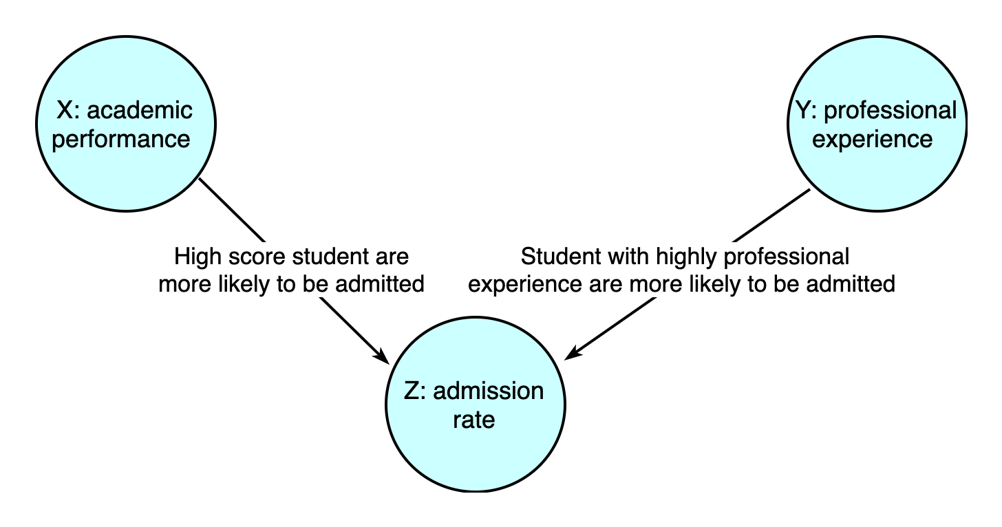
Suppose X and Y represent the academic performance and professional experience of a student, and we want to know if X has a causality on Y. Suppose the real situation is X and Y are independent. Also, there's a fact that students with high academic scores and outstanding work experience are more likely to be admitted by a university. Let Z donate the probability of a student being admitted by a university, the true causal structure of the problem is:

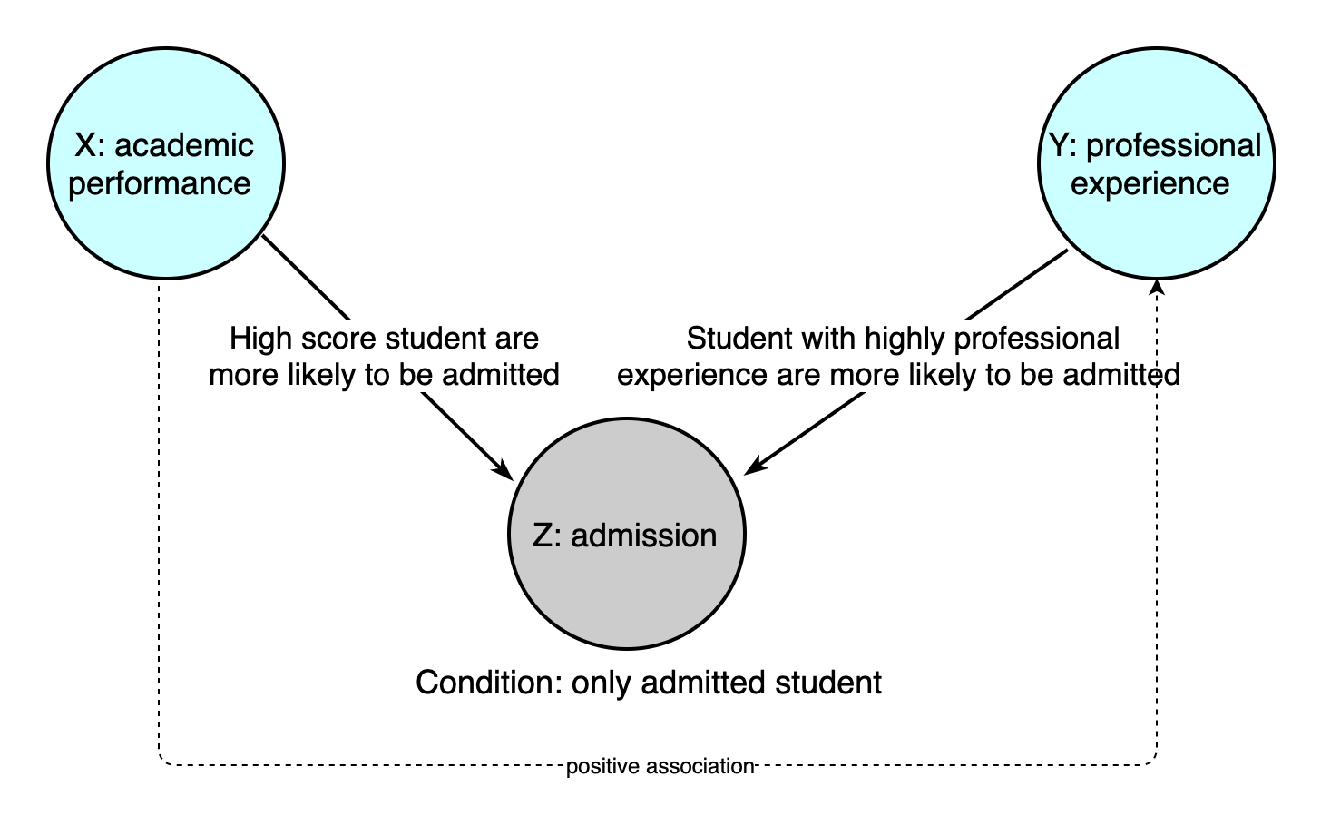
However, we failed to recognize such a variable Z that both caused by X and Y. When we draw the sample, we go to a university to investigate the academic performance and professional experience of its students. Thus, all samples drawn are student admitted by university.

To make it easy, consider X, Y and Z as binary variables. Suppose we have following data:

	Y = high	Y =low
X = high	\(\frac{130}{150}\)	\(\frac{40}{155}\)
X= low	\(\frac{50}{155}\)	\(\frac{5}{150}\)

In each cell, the numerator and the denominator respectively represent the number of admitted students and all students. Its easy to find that X and Y are independent by conducting a \(\chi^2\) test based on the denominator values.

Suppose there exists no confounders. The real ATE should be: \[ E[Y|X= high] - E[Y|X=low] = (150+155) - (155+150) = 0 \] However, as we conditioned on Z, the ATE we know observed become: \[ E[Y| X =high, Z = admitted] - E[Y|X=low,Z = admitted] = (130-40)-(50-5) = 45 \] We draw incorrect conclusions that X have positive causal effects on Y. The reason is that the the admitted student cannot represent the whole population. In this case, Z is a selection variable, it is caused by both X and Y. If we condition on Z, then association is created between X and Y, and we cannot accurately estimate the causal effect from X to Y through statistical dependency. This is called a selection bias.

2.3 Reverse Causation

Suppose we want to discover the causal relationship from longer marriage to longer life. The truth is that having a longer marriage has no positive on one's longevity. However, on the other hand, elder people usually have longer marriage as they spent more time. Thus, the true causal relationship between X(longevity) and Y(marriage length) is:

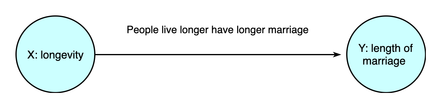
However, according to our assumption, the causality is reversed, we expected to test the following structure:

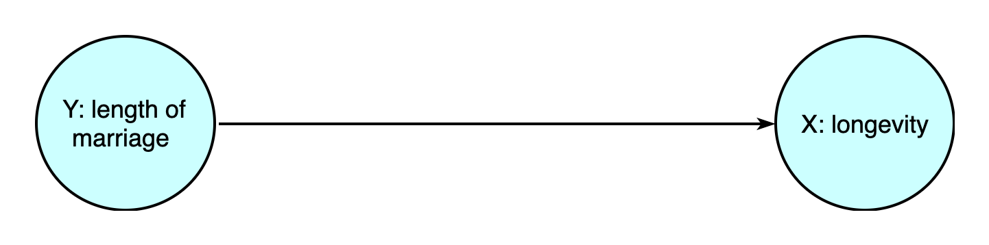
without any doubts, we would find a statistical dependency between X and Y as statistical association is not directed. However, letting people have longer marriage does not help extend thei lifetime. The causality we discovered is wrong as it is reversed.

3. Basic Methodology of Causal Inference

3.1 Experimental data and Observational Data

Observational Data

Data are observed and collected for each subjects. No manipulations(intervening) on these subjects occur. We can condition on certain variables, but what we have would then be a subset of the original data

Experimental Data

Subjects are manipulated(intervened). The mechanism the data generated are artificially changed.

Causal inference is very easy on experimental data, while can be much more difficult on observational data.

3.2 Randomized Control Experiment

We can estimate causality based on Experimental Data through Randomized Control Experiment(RCT).

Suppose we want to explore the causal relationship from increasing exercise to physical health. Let

• T: denote whether increase exercise
• Y: physical condition of a unit
• X: any confounder that can create a statistical correction between T and Y, such as gender, weight and age
• Z: any common results of Y and T, such as physical condition evaluation score

To collect observational data, we just record the T, Y and X of units we can observed

To collect experimental data, we need to split all subject into treatment group(increase exercise) and control group(not increase exercise). The process of deciding which group to assign for a subject should be completely randomized. This means X should have same distribution for treatment group and control group. We can such a scenario Covariate Balance \[ P(X|T=1)=^d P(X|T=0) \]

Under such intervention, we can regard as the causality from X to T are blocked(cannot demonstrate dependency). Also, such a randomized selection ensure that there's no conditioning on Z.

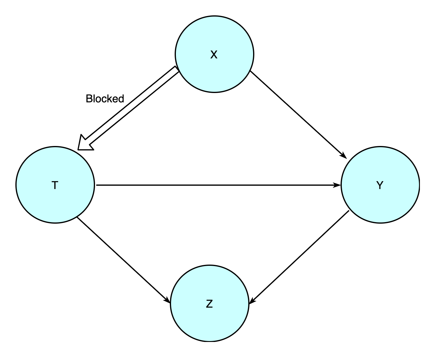
The randomized process ensured there's no other floating association from T to Y other than the directed chain path, which is the one we care about. Under this scenarios, we can estimate causal effect directly from