Evaluation Method for Classification

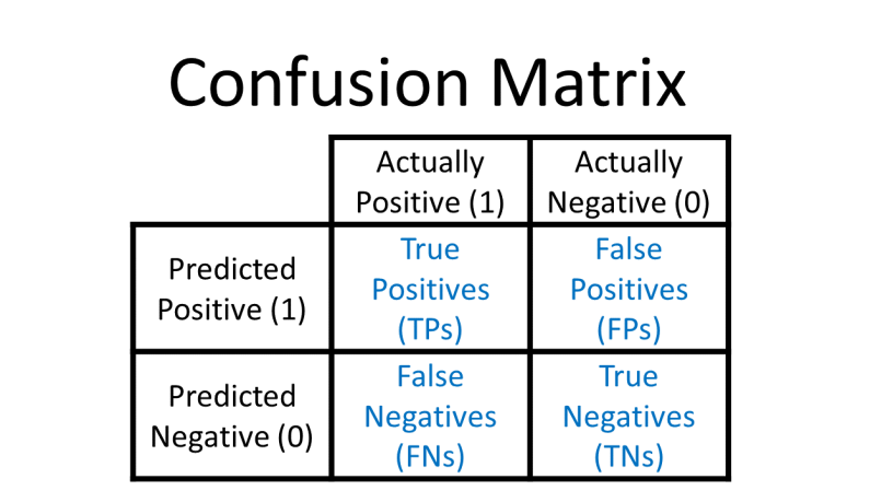
1. Confusion Matrix

The confusion matrix is a table that count different cases of the predicted outcome given by a classification model. For a binary classification model, it can be given as:

For a multiple classification case, the confusion matrix can be given as:

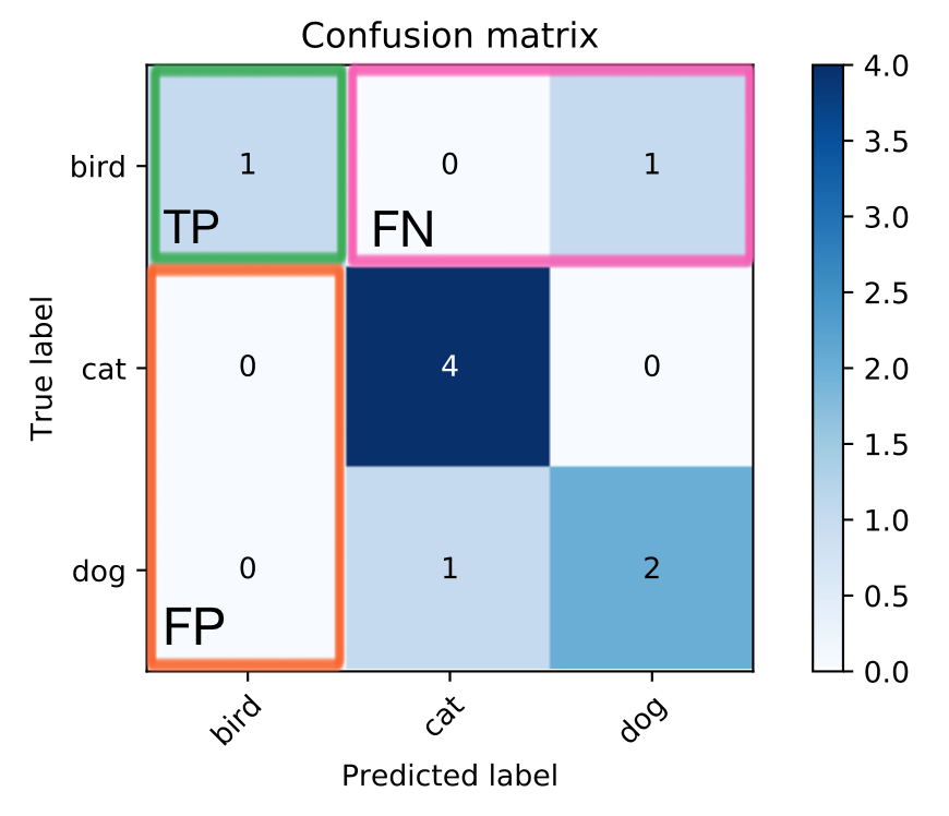
For such case, we can define TP, TN, FP, FN for each category by deeming all true “not-bird” samples predicted “not-bird” as TN, etc.

2. Accuracy, Precision, Recall and F1 score

With confusion matrix given, we can now define the following matrix:

Accuracy

Accuracy = samples predicted correctly / all predicted samples \[ accuracy = \frac{TP+TN}{TP+FP+FN+FP} \] Accuracy is a very intuitive metrics. However, it sometimes cannot directly reflect the predicting performance of the model as it cannot deal with imbalanced data. For example, suppose we have a sample set of 100 sample with 99 positive and 1 negative, even if the model simply predicted all samples as positive without any training, it would still receive an accuracy of 99%.

Recall and Precision

Recall = correctly predicted positive samples / all actual positive samples \[ racall = \frac{TP}{TP + FN} \] Recall represent the ability to find positive samples among all actual postive samples. It can deal with imbalanced data. It is sensitive to FN case, thus is suitable for the business case where FN would bring significant cause(e. g Explosion recognition, vehicle safety judgement). On the other side, recall does not consider FN, a model can simply improved recall by judging all samples as positive, which is not good in some cases.

Precision = correctly predicted positive samples / all predicted positive samples \[ precision = \frac{TP}{TP + FP} \] Precision represent the probability that a model's judgment on positive case is correct. It can partly deal with imbalanced data. It is sensitive to FP case, thus is suitable for the business case where FP would bring significant cause(e. g Crime judgment, disease diagnosis).

Recall and Precision can both deal with imbalanced data. However, there's a trade-off between these two metrics. Thus, which metric to put emphasis on idepends on specific business application. Nevertheless, in most cases, since we can just flip P/N, or 1/0, precision is more like an accompanied constraint of recall to prevent model from foucsing too much on capture the minor category samples, as FN and FP are both bad in most business application.

F1 Score

The F-measure is a function that balance Precision and recall \[ F_\alpha = \frac{(1+\alpha^2)*P*R}{(\alpha^2*P)+R} \] when \(\alpha\) = 1, we call this metric F1 score: \[ F1 = \frac{2PR}{P+R} \] F1 socre combine Recall and Precision to find a balance. It is suitable for many business case where we cannot decide a clear preference.

3. P- R Curve, ROC Curve and AUC

P- R Curve

P-R Curve is a curve to depict the relationship between Precision and Recall. It's application is similar to F1 score, but lessly used as F1 score is more concise to read( The higher the better)

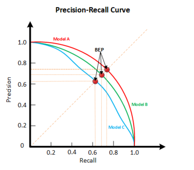
Usually, we can regard model B as a better model if it can completely wrap the curve of A. If that; s not the case, we can mark the point on the curve where precision equals recall(Break Event Point, or BEP). The curve with a BEP closer towards up- right direction is better.

ROC Curve

We define:

• True positive rate (sensitivity): the ratio that actual positive samples predicted correctly
• True negative rate (specificity): the ratio that actual negative samples predicted correctly
• False positive rate (1-specificity): the ratio that actual negative samples predicted wrongly

\[ TPR = \frac{TP}{TP+FN} = Recall \\ TNR = \frac{TN}{FP+TN} = 1-TNP \\ FPR = \frac{FP}{FP+TN} \]

From a probabilistic aspect:

Precision	\(P(Y=1|\hat{Y}=1)\)
Recall (sensitivity)	\(P(\hat{Y}=1|Y=1)\)
Specificity	\(P(\hat{Y}=0|Y=0)\)

From this interpreation, we found that sensitivity and specificity are condition on Y, which means The influence of P(Y) are blocked whe calculating these two metrics. Therefore, these two metrics are not influenced by the imbalance of data.

The Reciever Operating Characteristics cureve(ROC curve) take both metrics into consideration by depict the relationship between sensitivity and 1-specificity:

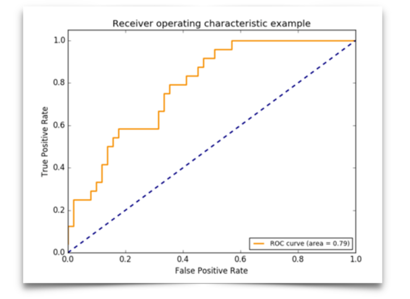
AUC

Area Under Curve(AUC) is the area beneath the ROC curve.

Suppose our model completely randomly classifies the samples, the the probability it regard an actual postive sample or an actual negative sample as a positive sample is equal, in this case, AUC would be 0.5. If AUC > 0.5, it means when the model predicts a sample, \(P(\hat{Y}=1|Y=1) > P(\hat{Y}=1|Y=0)\) , which means the prediction is effective. Thus, the higher the AUC is, the better the model performs.

Obviously, AUC is not influenced by imbalanced data, and it's delivery information concisely. Thus, it is one of the most frequently used metrics in classification.