Hypothesis Testing
Hypothesis Testing
1. Definition and Terms
Hypothesis testing is a kind of statistical inference method.
| Term | Meaning |
|---|---|
| Hypothesis | A claim to test |
| Null Hypothesis (\(H_0\)) | Currently accepted value for a parameter(e.g diff = 0) |
| Alternative Hypothesis(\(H_a\)) | The claims to be tested. \(H_0\) and \(H_a\) are mathematically opposites |
| Test Outcomes | Reject \(H_0\) or fail to reject \(H_0\) |
| Test Statistics | Statistics calculated from the data samples used to decide whether to reject \(H_0\) |
| Big/Small Sample | sample size -> inf / sample size is fixed, usually set threshold to 30 |
| Central Limit Theorem | A theorem that indicates no matter what distribution the total population is, when sample size n is big enough, the average of a statistics of a sample \(\bar{X}\) follows a normal distribution N(\(\mu\), \(\frac{\sigma^2}{n}\)). This theorem allows implementation of T- test on average of continuous test statistics, like average salary of a department |
| Degree of Freedom | The number of samples(n) -1 |
| Effect Size | The degree the test statistics differ from the accepted value |
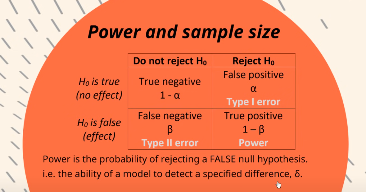
| Significance Level(1-\(\alpha\)) | A decided threshold of \(\alpha\). \(\alpha\) is the probability of rejecting \(H_ 0\) when \(H_ 0\) is ture(Type I Error) |
| Confidence Level | How confident we are to reject \(H_0\) (1-\(\alpha\)) |
| p value | The probability that the observed statistics significance are caused by random factor |
| statistical power(\(1-\beta\)) | \(\beta\) is the the probability of accepting \(H_ 0\) when \(H_ 0\) is False(Type II Error). Typically we need the power of a test to be greater than 80% |
| Confidence Interval | With \(\alpha\) as significance level, \(\theta\) as test statistics, if \(P\{ \theta_n < \theta < \theta_m \} \ge 1-\alpha\), then we call \((\theta_n , \theta_m)\) the confidence interval of \(\theta\) uhder the significance level \(1-\alpha\) |
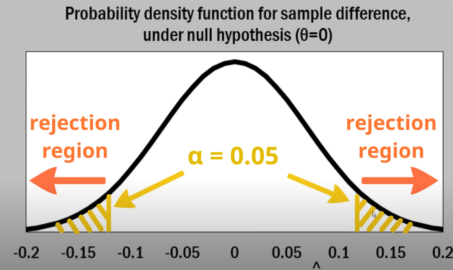
| One-tail Test/Two-tail Test | In one-tail test, the \(H_a\) has direction, so \(H_a\) would be like \(\mu > x\), and we only focus on one side of the rejection area in this case. While in two tail test, \(H_a\) would be like \(\mu \ne x\) |
| Rejection Area | Let the the area of PDF on \((-inf,z_1],[z_2,inf)] = \alpha\), then this area is called rejection area, \(b_0,b_1\) are called rejection boundaries, which are the z-score when the area one the left/right side is \(\frac{\alpha}{2}\). When the test statistics fall outside the rejection boundaries, we can reject \(H_0\) under the Level of Significance |
| MDE | The minimum detectable effect size of a experiment when \(1-\alpha\) and \(\beta\) is given. If detected effect size \(d < mde\), it might be caused by random factor, and we cannot reject \(H_ 0\) |
| PSB | Practical Significance Boundary |
Power and Error
2. Basic Procedure of Hypothesis Testing
2.1 Propose Hypothesis
Clarify the null hypothesis and alternative hypothesis to test on
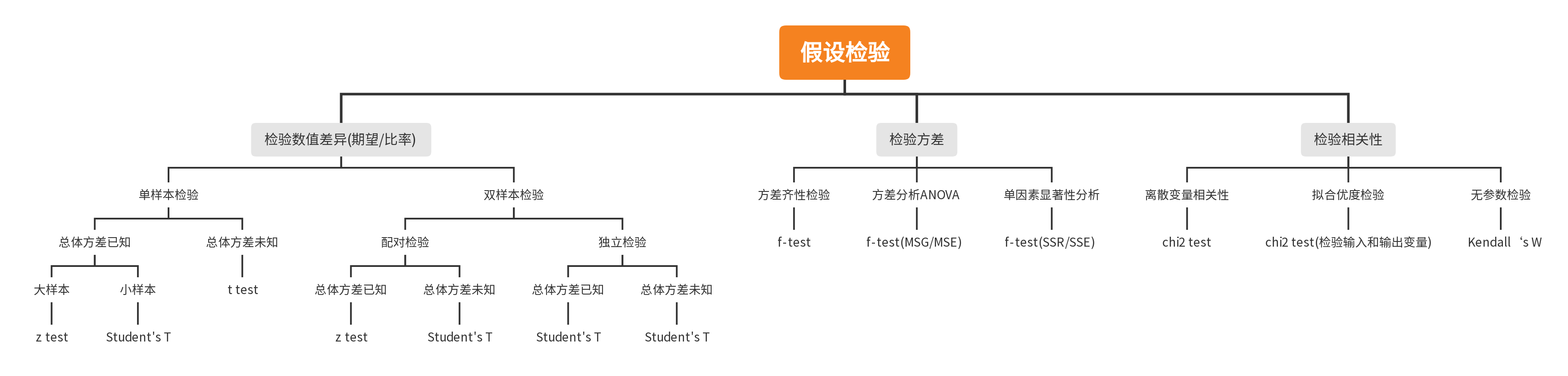
2.2 Test Type
2.3 Construct Test Statistics
For differential test, we usually want to test the difference between a parameter. In most case, we want to test the statistics based on a normal distribution. To do so, we would aggregate the measure though an additive way so that the parameter follows a normal distribution no matter what type of distribution the original measure follows. Thus, the parameter can should be concluded into 2 types: mean and ratio.
Since the parameter follows the normal distribution, we can construct the test statistics through Cohen's d: \[ d = \frac{(\theta_1-\hat{\theta_1})-(\theta_2-\hat{\theta_2})}{\sigma_{SE,pooled}} \] where \(\sigma_{SE}\) measures the variance of a parameters \(V[\theta]\).
For a mean test, \(\theta\) is a mean \(\bar{ X }\) \[ V[\bar{X}] = V[\frac{(X_1+X_2+...X_n)}{n}] = \frac{1}{n^2}\sum_i^nV[X_i]=\frac{1}{n}V[X_i] = \frac{\sigma^2_X}{n} \] For a ratio test, \(\theta\) is a ratio R \[ V[R] = V[\frac{B_1+B_2+...+B_n}{n}] = \frac{1}{n^2}\sum_i^nV[B_i]=\frac{1}{n}p(1-p) \] The calculation of pooled standard error would be discussed in the following sections
For ratio test, there's also another way to construct the test statistics called Cohen's h: \[ h = 2(arcsin \sqrt{p1} - arcsin\sqrt{p2}) \] For the correlation test between categorical variable, we can use Cramer's V to construct the test statistics \[ V = \sqrt{\frac{\chi^2/n}{min(c- 1,r-1)}} \]
2.4 Decide Testing Parameters
Significance Level
Decided by the preset \(\alpha\) in the testing. \(1-\alpha\) is the significance level, represent the strictness degree on judging significance.
Statistical Power
Decided by the preset \(\beta\) in the testing. Statistical Power represents the probability of rejecting \(H_0\) if it is indeed false, in other word, the probability of avoiding type II error. For example, in an one-tail differential Z test, let \(\beta'\) denote the real-time statistical power: \[ \beta' = P(d \le Z_{1-\alpha/2}|H_0 \ False) = P(\frac{\theta_1 - \theta_2-\Delta}{\sigma_E} \le Z_{1-\alpha/2} - \frac{\Delta}{\sigma_E}) \] where \(\Delta = \theta_1 - \theta_2\) is the real differential that exists. Let \(Z = \frac{\Delta}{\sigma_E}\) \[ 1 - \beta' = 1-\Phi(Z_{1-\alpha/2}-Z) = \Phi(Z- Z_{1-\alpha/2}) \] For a two-tail Z test: \[ 1 - \beta' = \Phi(Z- Z_{1-\alpha/2}) + \Phi(-Z-Z_{1-\alpha/2}) \]
Practical Significance Boundary
The preset \(\delta\) decided based on business goal. It is the minimum level of difference on metrics that we cares about. The PSB serve as an initial MDE used to decided minimum sample size.
Vairance of Population: The estimation on \(\sigma^2\) from the historical data of the population
Estimate the sample size
From the definition of the statistical power we can find that the minimum sample size required is associated with the expected statistical power. Given a fixed sensitivity(MDE), the higer power we want, the more sample we need. We can deduce the formula of minimum sample size as follows:
Mean Test: \[ n' = \frac{(\sigma_1^2+\sigma_2^2)(z_{\alpha/2}+z_{\beta})^2}{\delta^2} \] Ratio Test: \[ n'= \frac{Z_{\alpha/2}\sqrt{\frac{p_1+p_0}{2}(1-\frac{p_1+p_0}{2})}+Z_\beta\sqrt{p_1(1-p_1)+p_0(1-p_0)}}{p_1-p_0} \]
- where \(p_0\) is the baseline of the ratio
- \(p_1\) is the expected level of the ratio, \(p_1 = p_0 + \delta\)
2.5 Results Analysis
After the testing duration is reached, we can decide whether there is a statistical significance. Examine the p value of the observed results. If \(p < \alpha\) reject the Null hypothesis.
Also, check the sensitivity(the real-time mde). If the mde is greater than the preser \(\delta\), it is likely that the testing is underpower and needs more samples.
TO calculate real-time MDE \[ MDE = (t_{\frac{1-\alpha}{2}} + t_ {1-\beta})\sqrt{\frac{s_1^2}{n_ 1} + \frac{s_2^2}{n_ 2}} \]
According to the definition of the statistical power, the sensitivity of the testing is associated with the preset statistical power.
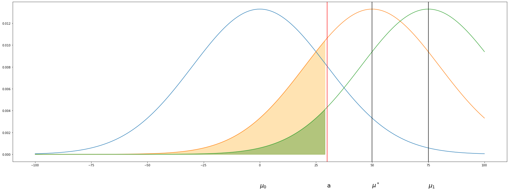
In the this figure
- the orange area is the preset \(\beta\)
- the green area represent the true type II error \(\beta'\)
- \(\mu_0\) is the mean of the test statements under \(H_0\), which is 0
- \(\mu^*\) is the mean where the statistical power is exactly \(1-\beta\). \(\mu^*\) decides the MDE of the experiment
- \(\mu_1\) is the true value of the statistics estimated from the sample
From the figure we can find out that if the true difference is bigger than MDE, than the ture statistical power is greater then we demands, and the experiment is overpowered. On the opposite, if the true difference is smaller than the MDE, than we cannot detect the difference with enough power, and the experiment is underpowered
When the sample size remains the same, higer power, which means lower type II error, demands the right-forward shift of mean of the parameter and leads to greater mde(lower sensitivity). If we want to improve sensity while maintaining the power, we would need more samples or find a way to lower the variance of the metrics
3. Z/T-test
Z Test:
A Z-test examine a statistics assuming it follow a standard normal distribution(distribution). Thus the construction of z statistics is \(Z = \frac{X-\mu}{\sigma}\)
T-test
A T-test construct a statistics like: \(t = \frac{X}{\sqrt{Y/n}}\) where \(X\sim N(0,1)\) and \(Y \sim \chi^2(n)\) . In a mean test \(\sqrt{Y/n}\) could be the standard error. The advantage of T test is, while it have similar testing capability as Z test when n is greater than 30, it does not require the population variance \(\sigma\) to be given. Meanwhile, it has stronger testing capability when n is smaller than 30
3.1 One Sample Test
Objective: to test whether the accepted mean or ratio of a population is correct through a sample. In this case, we can assume \(\mu_0\) and \(\pi_0\) is given
3.1.1 \(\sigma\) Given(T or Z)
In most application, the standard deviation of the whole population is unknown. But suppose we have the \(\sigma\)
Big Sample
For big sample, we conduct z-test and give hypothesis as:
\(H_0: \mu = \mu_ 0\) or \(\pi = \pi_0\) for ratio test
\(H_1: \mu \ne \mu_ 0\) or \(\pi \ne \pi_0\) for ratio test
where \(\mu_0\) is the accepted value of the parameter and construct z-score as: \[ z = \frac{\bar{x}-\mu_0}{\sigma/\sqrt{n}} \] for ratio test, construct z as: \[ z = \frac{p-\pi_0}{\sqrt{\frac{\pi_0(1-\pi_0)}{n}}} \] Small Sample
When the sample size is small, we can assume the sample ~ t distribution. The construction of the test statistics and reject condition are the same, the only difference is that the test statistics is now following t distribution
3.1.2 \(\sigma\) Unknown(T)
When \(\sigma\) is unknown, the basic strategy is to replace population std with sample std, and apply t-test
We can conduct t-test and give hypothesis as:
\(H_0: \mu = \mu_ 0\) or \(\pi = \pi_0\) for ratio test
\(H_1: \mu \ne \mu_ 0\) or \(\pi \ne \pi_0\) for ratio test \[ t = \frac{\bar{x}-\mu_0}{s/\sqrt{n}} \] for ratio test, construct t as: \[ t = \frac{p-\pi_0}{\sqrt{\frac{\pi_0(1-\pi_0)}{n}}} \]
3.2 Two Sample Test
Objective: to test whether a condition would effect a metric through following one group before and after experiment or comparing two groups
3.2.1 Match Test
Usually applied when testing treatment on a same group of people in different time(e. g medical treatment). In this context, we can assum the sample size and standard deviation remain as same: \(n_ 1 = n_ 2, \sigma_1 = \sigma_2\)
3.2.1.1 \(\sigma\) Given(Z)
\(H_0: \mu_1 = \mu_ 0\) or \(\pi_1 = \pi_0\) for ratio test
\(H_1: \mu_1 \ne \mu_ 0\) or \(\pi_1 \ne \pi_0\) for ratio test \[ z = \frac{(\bar{x_1}-\bar{x_0}) - (\mu_1-\mu_0)}{\sigma\sqrt{\frac{2}{n}}} = \frac{\bar{d}}{\sigma\sqrt{\frac{2}{n}}} \] for ratio test, construct z as: \[ z = \frac{(p_1-p_0) - (\pi_1 - \pi_0)}{\sqrt{p(1-p)(\frac{2}{n})}} \]
\[ p = \frac{p_0+p_1}{2} \]
3.2.1.2 \(\sigma\) Unkown(T)
\(H_0: \mu_1 = \mu_ 0\) or \(\pi_1 = \pi_0\) for ratio test
\(H_1: \mu_1 \ne \mu_ 0\) or \(\pi_1 \ne \pi_0\) for ratio test \[ t = \frac{\sqrt{n}((\bar{x_1}-\bar{x_0}) - (\mu_1-\mu_0))}{s_d} = \frac{\sqrt{n}\bar{d}}{s_d} \] where \(s_d\) is the standard deviation of d
for ratio test, construct z as: \[ t = \frac{(p_1-p_0) - (\pi_1 - \pi_0)}{\sqrt{p(1-p)(\frac{2}{n})}} \]
\[ p = \frac{p_0+p_1}{2} \]
3.2.2 Independent Test
Usually applied when evaluation the effect of a treatment by comparing a experiment group and control group, which is A/B Testing
3.2.2.1 \(\sigma\) Given(Z)
\(H_0: \mu_1 = \mu_ 0\) or \(\pi_1 = \pi_0\) for ratio test
\(H_1: \mu_1 \ne \mu_ 0\) or \(\pi_1 \ne \pi_0\) for ratio test
if \(\sigma_1 = \sigma_2\) \[ z = \frac{((\bar{x_1}-\bar{x_2}) - (\mu_1-\mu_2))}{\sigma \sqrt{\frac{1}{n_1}+\frac{1}{n_2}}} \]
if \(\sigma_1 \ne \sigma_2\) \[ z = \frac{(\bar{x_1}-\bar{x_2}) - (\mu_1-\mu_2)}{\sqrt{\frac{\sigma_1^2}{n_1}+\frac{\sigma_2^2}{n_2}}} \] for ratio test: \[ z = \frac{(p_1-p_2) - (\pi_1 - \pi_2)}{\sqrt{p(1-p)(\frac{1}{n_1}+\frac{1}{n_2})}} \]
\[ p = \frac{p1*n1+p_2*n_2}{n_1+n_2} \]
3.2.2.1 \(\sigma\) Uknown(T)
\(H_0: \mu_1 = \mu_ 0\) or \(\pi_1 = \pi_0\) for ratio test
\(H_1: \mu_1 \ne \mu_ 0\) or \(\pi_1 \ne \pi_0\) for ratio test
if \(\sigma_1 = \sigma_2\) \[ t = \frac{((\bar{x_1}-\bar{x_2}) - (\mu_1-\mu_2))}{s_p\sqrt{\frac{1}{n_1}+\frac{1}{n_2}}} \]
\[ s_p = \sqrt{\frac{(n_1-1)s_1^2+(n_2-1)s_2^2}{n_1+n_2-2}} \]
if \(\sigma_1 \ne \sigma_2\) \[ t = \frac{((\bar{x_1}-\bar{x_2}) - (\mu_1-\mu_2))}{\sqrt{\frac{s_1^2}{n_1}+\frac{s_2^2}{n_2}}} \] for ratio test: \[ t = \frac{(p_1-p_2) - (\pi_1 - \pi_2)}{\sqrt{p(1-p)(\frac{1}{n_1}+\frac{1}{n_2})}} \]
\[ p = \frac{p1*n1+p_2*n_2}{n_1+n_2} \]
4. F-test
An F-test construct the test statistics like \(\frac{U_1/d_1}{U_2/d_2}\), where \(U1 \sim \chi^2(d_1)\) and \(U_2\sim \chi^2(d_2)\). In testing for Equality of Variances, the \(\frac{U}{d}\) can be the standard error
4.1 Equality of Variances
Through F-test, we can examine the equality of the variances of two normally distributed varaible
Let \(X_1,X_2\) be two independent variables, where: \[ X_1~N(\mu_1,\sigma_1^2), X_2~N(\mu_2,\sigma_2^2) \] Get a sample from each variable: \(x_1, x_2\), the sample sizes are \(n_1,n_2\)
Let \(\bar{x}_1,\bar{x}_2\) be the mean of the samples, \(s_1,s_2\) be the standard error of the samples
Set the null hypothesis and alternative hypothesis of Experiment: \[ H_ 0: \sigma_1^2 = \sigma_2^2\\ H_ 1: \sigma_1^2 \neq \sigma_2^2 \] If it is a one-tail experiment: \[ H_ 0: \sigma_1^2 < \sigma_2^2\\ H_ 1: \sigma_1^2 \ge \sigma_2^2 \]
Construct F statistics: \[ F(n_1-1,n_2-1) = \frac{s_1^2/\sigma_1^2}{s_2^2/\sigma_2^2}=\frac{s_ 1^2}{s_2^2} \] Note: As a convention, we normally select the greater s as \(s_ 2\) to let f score <1
Look up the F score table, if \(F > F_{\alpha}\), reject \(H_0\)
If it is a one-tail experiment, then reject \(H_0\) when \(F < F_{1-\alpha}\)
4.2 Single Factor ANOVA
We can use f- test to examine the impact of a factor to an indicator by judging if the indicator is same when the factor is set to different value
Let the factor be X, indicator be Y. Let SST denote the total variance of Y, SSA denote the variance between groups grouping by value of X, SSE denote the variance of Y within each gropu, we have: \[ SST = SSA + \sum_ i SSE_i \]
Suppose we got the following observations:
| X = \(x_1\) | X = \(x_2\) | X = \(x_3\) | X = \(x_4\) |
|---|---|---|---|
| y=1 | y=2 | ... | ... |
| y=3 | y=3 | ... | ... |
| y=2 | y=4 | ... | ... |
| y=6 | y=6 | ... | ... |
Let k = number of groups(number of different values of X), \(n_i\) = the number of samples in \(i_{th}\) group, n = \(max(n_ k)\)
Construct F statistics \[ F = \frac{SSA/df1}{SSE/df2} \] With:
\(df1 = k - 1\)
\(df2 = n- k\)
SSA is Sum of Square Between Groups:
\[ SSA = \sum_{i=1}^kn_i(\bar{y_i}-\bar{y}) \] Where:
- \(\bar{y_i}\) is the average of the \(i_{th}\) group
- \(\bar{y}\) is the average of all \(\bar{y_i}\)
SSE is the Sum of square error \[ SSE = \sum_{i=1}^k(n_i-1)s_i^2 \] Where:
- \(s_1^2\) is the variance(square of standard error) of the \(i_{th}\) group
Look up the F score table, if \(F > F_{\alpha}\), reject \(H_0\)(the factor do has an impact)
4.3 Linear Regression ANOVA
We can use f-test to examine on whether a liner model(linear hypothesis) fit a problem well
Suppose we got the following linear hypothesis function: \[ y = \beta_ 0+\beta_1x_1 + \beta_2x_ 2 +... \beta_mX_m +\epsilon \] For a regression model, we believe there's such a equitation: \[ \begin{aligned} TSS &= ESS + RSS\\ \sum_i^n(y_i-\bar{y})^2 & =\sum_i^n(\hat{y_i}-\bar{y})^2+\sum_i^n(y_i-\hat{y_i})^2 \end{aligned} \] In this equations, TSS stands for the total sum of squared error, which is the variance of the output variable. ESS stands for the explained sum of squared error, which represents estimated variance of Y, ot to say, the variance explained by the model. The RSS stands for the residual sum of squared error, which represents the error casued by the model's failure to capture the pattern. If \(ESS = 0\), TSS = RSS, which means the model equals to a model that simply predicted all samples as the average of Y, which indicates the model has a bad performance.
With null hypothesis \(H_0: \beta_1 = \beta_2=...=\beta_m = 0\), or we can say \(H_0: ESS = 0\), we construct F statistics as: \[ f = \frac{ESS/df_{ESS}}{RSS/df_{RSS} } = \frac{ESS/m}{RSS/(n-m-1)} \] where:
n is number of samples
m is number of variables(x)
Look up the F score table, if \(F > F_{\alpha}\), reject \(H_0\). In such case, the variance of Y can be well explained by the variance of X. Otherwise, consider feature engineering or a non-linear model.
5. \(\chi^2\) Test
A \(\chi^2\) Test construct the test statistics as a function of a \(\chi^2\) variable. The degree of freedom are usually involved in the construction of such a statistics
5.1 Chi-squared Test for Independence
chi-squared test is a supervised hypothesis testing method to calculate the probability that 2 categorical variables are correlated
Suppose there are categorical variables X and Y, X has r possible values, with probability \((p_{x,1},...p_{x,r})\) and Y has c possible values, with probability \((p_{y,1},...p_{y,c})\).
Under the null hypothesis, since X and Y are independent, the probability of observing \(X=c_{x,i}, Y = c_{y,j}\) would be \(p_{i,j} = p_{x,i}p_{y,j}\)
In such case, let \(t_{i,j}\) be the observed times that \(X=c_{x,i}, Y = c_{y,j}\), t would follow a binomial distribution \(Bin(t;n,p_{ij})\)
According to properties of binomial distribution, when n is big enough, \(Bin(t;n,p_{i,j})\) is approximately \(N(np_{i,j},np_{i,j}(1-p_{i,j}))\)
According to the definition of \(\chi^2\) distribution, let \[ \chi^2=\sum_i^r\sum_j^c \frac{(t_{i,j}-E[t_{i,j})^2]}{E[t_{i,j}]} \] \(\chi^2\) would follow a \(\chi^2\) distribution, with the degree of freedom being \((r-1)(c-1)\)
We can calculate the \(\chi^2\) and obtain its according p value through p value table for \(\chi^2\) distribution. If p < 0.05, we can reject the null hypothesis that the two variables is independent
Note that in a \(\chi^2\) testm the probability \((p_{x,1},...p_{x,r})\) and \((p_{y,1},...p_{y,c})\) is not a hypothesis to test, it is a believed fact. In real application, it needs to be estimated from observations. When number of observations is big enough, the error of estimation can be ignored.
A example is given below:
According to the observations, make the frequency table
calculate the row total and the column total
calculate the expectations for each cell by \(\frac{R_i*C_j}{total}\) (\(\frac{125*310}{600} = 65\),etc.)
the \(\chi^2\) would be \[ \chi_{i,j}^2 = \frac{(O_{i,j} - E_{i,j})^2}{E_{i,j}}\\ \chi^2 = \sum_{i,j}^{r,c}\chi_{i,j}^2 \]
movie type High POPULARITY low POPULARITY Row total type1 50(65) 75(60) 125 type2 125(155) 175(145) 300 type3 ... ... ... type4 ... ... ... column total 310 290 600 calculate the degree of freedom, \(k=(r-1)(c-1)\)
check the significance table of chi distribution to find the threshold of \(\chi^2\) given k and \(\alpha\)
compare the \(\chi^2\) with the rejection area, if \(\chi^2\) is greater than the threshold(which means p value is smaller than \(\alpha\)), then reject the null hypothesis
1 | |
5.2 Chi-squared Test for Goodness of fit
The process is basically the same.
| Category | Predicted times | Observed time |
|---|---|---|
| C1 | ... | |
| C2 | ||
| C3 |
Construct the \(\chi^2\) as: \[ \chi^2 = \sum_i^k\frac{O_i-P_i}{P_i} \] the \(\chi^2\) follows a \(\chi^2(k-1)\) when number of observations is big enough