Basic Statistics for Data Science
Statistics for Data Science
1. Basic Concepts for Statistics
Statistics: Statistics gather, describe and analyze sample data in a numerical way to understand the whole population
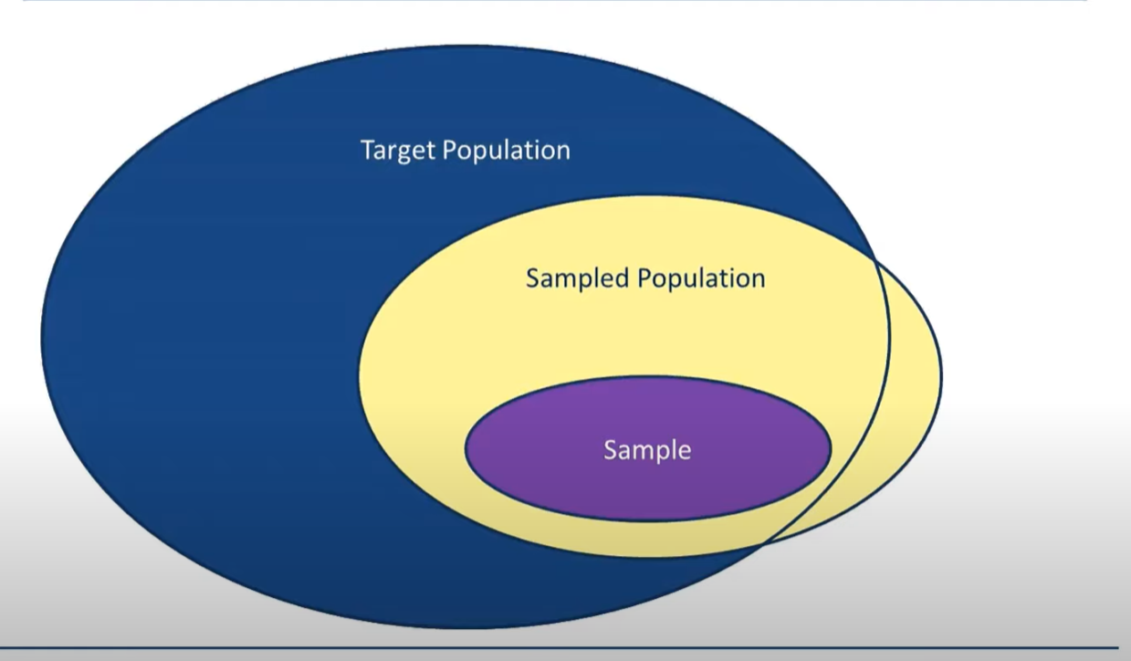
Target Population: A particular group of interest, the distribution of the target population is called
Sample Population: A group which the sample is taken from. In most cases it equals to the target population
Sample: A subset of the sample population from which data are collected, Doing statistics is a process trying to learn information of the target population through samples. Ideally, sample should be representative to sample population, the sample population should be the same or representative to target population.
Variable: A dimension of a sample representing a specific measure. A sample can contain multiple variables
Data : the actual counts, measurements or observation about the variables that markdown with samples
Data Point and Sample Size: Data point is a single record of data in the sample. Sample size is the number of data point in the sample
Parameter: A numerical description of a population characteristic. Note that a parameter of target population and sample is not the same. We cannot construct statistics with unknown parameters of the whole population
Sample Statistics: A function constructed from the sample. A statistics should containing no unknown parameters. Common sample statistics includes:
| Sample Statistics | Format |
|---|---|
| mean | \(\bar{X} = \frac{1}{n}\sum_i^nX_i\) |
| biased variance | \(S_0^2 = \frac{1}{n}\sum_i^n(X_i - \bar{X})^2\) |
| unbiased variance | \(S^2 = \frac{1}{n-1}\sum_i^n(X_i - \bar{X})\) |
| standard deviation | \(S = \sqrt{S^ 2}\) |
| moment | \(A_k = \frac{1}{n}\sum_i^nX_i^k\) |
| central moment | \(B_ k = \frac{1}{n}\sum_i^n(X_i - \bar{X})^k\) |
2. Data Classification
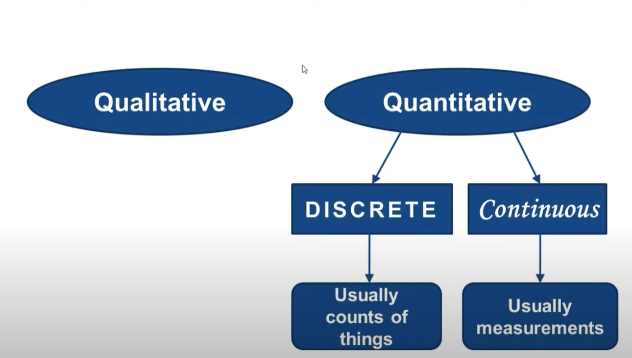
2.1 Categorical & Numeric
Categorical: consist of labels or description of traits. It's meaning less to apply quantitative calculation on it
Numeric: consist of counts and measurement, it have meanings when you apply quantitative calculations
2.2 Discrete & Continuous
Discrete: numeric data that can take only particular values(counts, rate stars)
Continuous: numeric data that can take any values in an interval
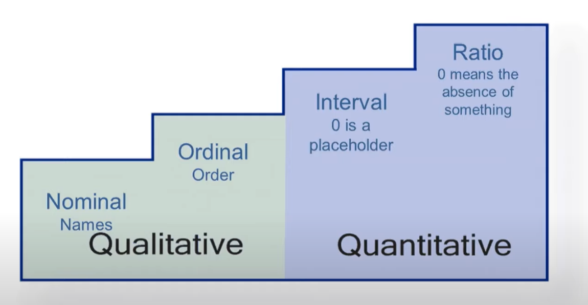
2.3 NOIR
Nominal level data: description of categorical data that order do not matters
Ordinal level data: categorical data that have a meaningful order(still not meaningful to add or divide)
Interval level data: numeric data that can be arranged in a meaningful order, and the different between data entries are meaningful(timestamp, shoe size, temperature degree)
Ratio level data: Interval data where zero indicates absence of something(like body height, 0 inch body high do not have a actual meaning, it means the data are not collected, where 0 degree do have an actual meaning, so it is not a ratio data.) As ratio data cannot participate calculation if data is not included, it must be non-zero in a calculation, thus it can divide other numeric data, that is why it is called ratio data
3. Two Important Theorem
There are two important probability theorem for statistics:
3.1 Law of Large Number
Chebyshev's inequality
For a random variable X, if E[X] and V[X] both exist: \[ P(|X-X[x ]| \ge \epsilon ) \le \frac{D[X]}{\epsilon^2} \] This inequality implies taht the probability of an observation fall far from the expectation is small. The greater \(\epsilon\) is, the smaller this probability is.
Chebyshev's Law of Large Number
Let a sequence \(X_n \to a\): \[ \lim_{n\to \infty} P(|X_n - a| < \epsilon) = 1 \qquad \forall \epsilon \] This law implies that a statistics on a sample would approaches the same statistics on the population as the sample size is big. In other word, the sample can represent the population when n is big.
3.2 Central Limit Theorem
If a random phenomenon is caused by numerous factors that have same distribution but are independent to each other, then the limit of thu sum of these factors, which is the phenomenon, follows a normal distribution.
The CLT can be expressed in the following format:
Lindeberg–Lévy CLT
Let \(X_1, X_2,..X_n\) be a series of independent random variables following same distribution, \(E[X_i] = \mu, V[X_ i] = \sigma^2\), then \[ \lim_{n\to \infty}P(\frac{ \sum_i^n X_ i-n\mu}{\sqrt{n}\sigma } \le X) = \Phi_0(X) \] where \(\Phi_0\) is a standard normal distribution
This theorem implies that when n is big enough, let \(Y = \sum_i^nX_i\), we can regarding Y as following a normal distribution \(N(n\mu, n\sigma)\)
Such a conclusion has very important meaning to hypothesis testing. It indicates that, if a statistics is constructed through through adding up sample point, lilke mean, then this statistics should follow a normal distribution no matter what distribution each sample follows. In hypothesis test, if we want to test on the mean of a measure of the population, we can regard that measure of each sample point as a random variable, these variables are independent and same-distributed, so no matter what distribution that measure follows, the mean of it on the total should follow a normal distribution. According to law of large number, as long as n is big enough, the mean on the sample should also follow normal distribution. Thus CLT make hypothesis testing on mean statistics possible.
Let \(\mu, \sigma^2\) be the mean and variance of the population, \(\bar{X},S^2\) be the mean and variance of the sample. According to Law of Large Number and CLT: \[ E[\bar{ X}] = \mu \]
\[ V[\bar{X}] = \frac{1}{n}\sigma^2 \]
\[ E[S^2] = \sigma^2 \]
4. Topic in Applied Statistics
Some topics in statistics are widely applied in domains like machine learning and A/B Test
1.Sampling
Sampling in statistics refers to the process of selecting a subset of individuals or observations from a population to estimate or infer the characteristics of the entire population. The goal of sampling is to obtain a representative sample that accurately reflects the characteristics of the population being studied.
For sampling sand simulation, refer to this article
2. Probability Density Estimation
Probability density estimation is a statistical technique that estimates the probability distribution of a random variable based on a set of observations. It is used to model the underlying probability distribution that generated the data.
For probability density estimation,refer to this article
3. Statistical Learning and Machine Learning
Statistical learning is a subfield of statistics that focuses on the study of learning algorithms and models. It involves the use of mathematical and computational techniques to infer relationships and patterns in data.
Machine learning is an engineering concept based on statistical learning. Statistical learning focuses more on inferring patterns between variables, while machine learning is more concerned with the effectiveness of the model in performing its function. In addition, the hypothesis space of machine learning is broader and does not necessarily have to be immediately derived from the perspective of probability distribution of data. Machine learning is a comprehensive discipline that integrates probability theory, statistics, optimization, computer science, and other fields.
For basics concept of machine learning,refer to this article
4. Experiment and Hypothesis Testing
Hypothesis testing is a statistical method used to determine whether a hypothesis about a population parameter is supported by the sample data. It involves setting up two competing hypotheses, the null hypothesis and the alternative hypothesis, and using sample data to determine which hypothesis is more likely to be true.
For hypothesis testing,refer to this article
5. Observational Study and Causal Inference
Observational study is a type of statistical study based on observational data rather then experimental data. Causal inference is the process of determining whether a cause-and-effect relationship exists between two variables. In observational studies, causality can be difficult to determine because of the potential for confounding variables.
For causal inference, refer to this article
6. Random Process
Stochastic processes are random processes that describe the evolution of a system over time. They are used in a wide range of fields, including physics, engineering, finance, and biology. A stochastic process is typically defined as a collection of random variables that evolve over time in some probabilistic manner.
7. Time-series Analysis
Time-series analysis is a statistical technique used to analyze and extract meaningful patterns and relationships in time-series data. This technique is widely used in various fields, such as finance, economics, weather forecasting, and signal processing. Time series analysis can help identify trends, seasonal patterns, and irregularities (such as outliers) in data. It can also be used to forecast future values based on historical data.