Feature Selection: Statistical Method

1. Filter

Evaluate features on divergence and correlation. set one or more thresholds and select the feature.

Pro: fast, scalable, independent of the model

Con: ignore the dependence of features

1.1 Variance/Skewness

For most models, variables with high variance or skewness would be weighted more and deemed as more important. Thus, we can

1. calculate the variance(not STD) of each feature
2. set a threshold, select all features whose variance bigger than the threshold

Calculation of Skewness: \[ SK = \frac{n\sum(x_i-\bar{x})^3}{(n-1)(n-2)\sigma^3} \] An implementation of feature selection based on variance in Python

from sklearn.feature_selection import VarianceThreshold
#threshold 是方差的阈值
#返回选择后的特征
data_1 = VarianceThreshold(threshold=0.25).fit_transform(data_0)

1.2 Correlation

1. calculate the correlation value between each feature and the target
2. select the features with top K biggest correlation value

1.2.1 Pearson R

Pearson R calculates correlation based on covariance. \[ p_{X,Y} = \frac{cov(X,Y)}{\sigma_X \sigma_Y} = \frac{E[(X - \mu_X)(Y-\mu_Y)]}{\sigma_X \sigma_Y} = \frac{E[XY]-E[X]E[Y]}{\sqrt{(E[X^2]-E[X])^2} \sqrt{(E[Y^2]-E[Y])^2}} \] For a sample with n samples: \[ r = \frac{\sum_i^n(X_i-\bar{X})(Y_i-\bar{Y})}{\sqrt{\sum_i^n(X_i-\bar{X})^2} \sqrt{\sum_i^n(Y_i-\bar{Y})^2}} = \frac{\sum XY - \frac{\sum X \sum Y}{n}}{\sqrt{\sum X^2 - \frac{(\sum X)^2 }{n}} \sqrt{\sum Y^2 - \frac{(\sum Y)^2 }{n}}} \] The Pearson R has following properties:

• The range of Pearson R is [-1,1], positive numbers indicate positive correlation
• The Pearson R represents the linear correlation between two variables, linear transformation of X or Y does not change Pearson R
• X and Y must be numerical variables and follow normal distribution
• The observations of X and Y are in pairs

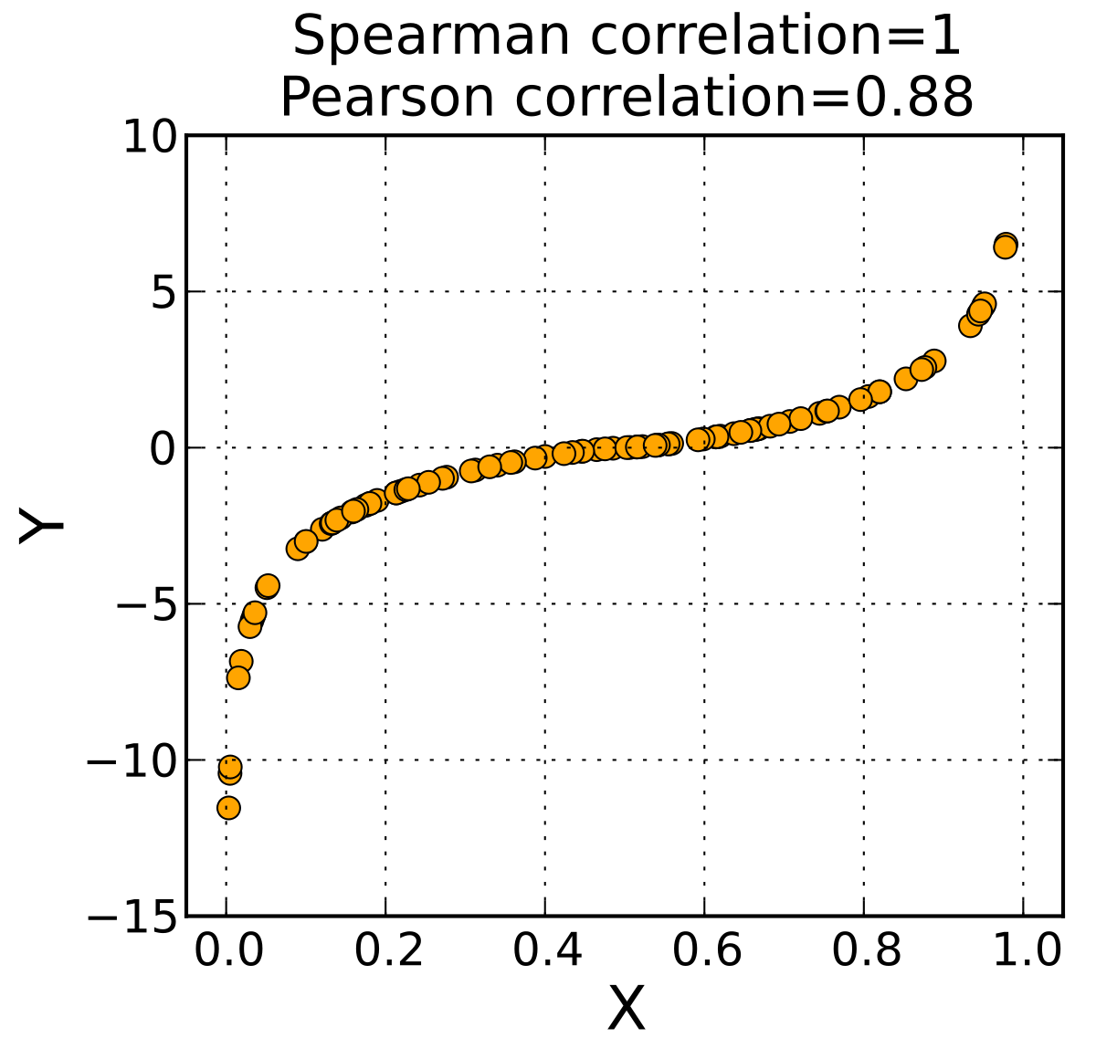
1.2.2 Spearman

Suppose we have samples of X and Y with n observations. Sort the observations X and Y to obtain two new set \(a\) and \(b\), where \(a_i,b_i\) is the rank of \(X_i,Y_i\) in X,Y

define Spearman correlation as: \[ \rho = \frac{6\sum_i^n(a_i-b_i)^2}{n(n^2-1)} \] The Spearman correlation has following properties:

• The range of Spearman correlations is [-1,1], positive numbers indicate positive correlation
• The Spearman correlation represents rank correlation (simply based on size relationship)
• X and Y does not need to follow certain distribution. Aithough the sample must be the same, they do not need to be in pairs
  
• The statistical power of Spearman is relatively lower

1.2.3 Kendall

Suppose we combine variables X and Y into a new element \((X,Y)\). If two elements \((X_i, Y_i)\) and \(X_j,Y_j\) satisfy either of these two case:

• \(X_i > X_j\) and \(Y_i >Y_j\)
• \(X_i < X_j\) and \(Y_i <Y_j\)

Then we call these two elements have consistency

if \(X_i = X_j\) and \(Y_i = Y_j\), we regard these two elements as having neither consistency nor inconsistency. Otherwise, we call these two elements have inconsistency

define Kendall correlation as: \[ \tau = \frac{C-D}{\sqrt{N3-N1}\sqrt{N_3-N_2}{}} \] where:

• C is number of paris of elements(Two element \((X _1,Y_1),(X_2,Y_ 2)\) is one pair) that have consistency

• D is number of paris of elements that have inconsistency

• \(N1 = \sum_i^s \frac{ 1}{2}U_i(U_i-1)\), where:

  • s is the number of values in X that appears more than once
  • \(U_i\) is the number those values appears(For \(i^{th}\) Values in s)
  • For example, for a X={1,2,2,3,3,3,4}, s=2, \(U_1 = 2, U_2 = 3\)

• N2 is calculated same way as N1 on Y

• \(N3 = \frac{1}{2}N(N- 1)\), where is the number of samples

The Kendall correlations have similar conditions as Pearson R. The only difference is it represents rank correlation instead of linear correlation

• The range of Pearson R is [-1,1], positive numbers indicate positive correlation
• X and Y must be numerical variables and follow normal distribution
• The observations of X and Y are in pairs

An implementation of feature selection based on Pearson R in Python

from sklearn.feature_selection import SelectKBest
from scipy.stats import pearsonr
def get_all_pscore(x,y):
    k = np.zeros([4,2])
    for i in range(0,x.shape[1]):
        temp = pearsonr(x[:,i],y[:,0])
        k[i,:] = np.array(temp)
    return [k.T[0],k.T[1]]
# 下面的写法有问题理论上应该与上面的函数等价，实际上在调用np.array时，会把最内层的pearsonr系数值变成一个数组对象，导致SelectKBest无法
# 遍历，需要用astype把第一列转化为float，但这样很难封装进lambda函数里，不如不用，写这个的人铁nt，害我研究一个多小时
# get_all_pscore =  lambda X,Y:np.array(list(map(lambda x:pearsonr(x,Y),X.T))).T

#第一个参数为一个callable()，该函数以feature，target为输入，输出可以是两种：
# 1. 一对数组pearsonr系数-p值（可以是tuple中两个数组，也可以是ndarray，总之第一个维度须为2
# 2. 一个单一的数组（只有相关系数）
# 第二个参数k，代表选择前k个
data_1 = SelectKBest(get_all_pscore(),k=2).fit_transform(data_0,target_0)

1.3 Hypothesis Testing

We can conduct hypothesis testing on correlation to examine whether the correlation of two variables are significant, and we can drop those features with high correlation with others.

For example, we can conduct \(\chi^2\) test to test the correlation of discrete variables. We can conduct Fisher's Z test on the correlation coefficient to determine whether the correlation are significant.

For details of these tests, refer tothis article

1.4 Mutual Information

For the theoretical part about Entrophy and Mutual Information, refer to this article \[ MI = H(x,y) - H(x|y) - H(y|x) = \sum_x\sum_yp(x,y)log\frac{p(x,y)}{p(x)p(y)}\\ \] Suppose we have an input variable X with n samples and m unique values {\(x_1 = c_ 1,x_2 =c_ 1,...x_n = c_m\)} and an output variable Y with n samples and k unique values {\(y_1 = c_ 1,y_2 =c_ 1,...y_n = c_k\)}

It's easy to calculate \(P(X=c_i),P(Y=c_j),P(X=c_i,Y=c_j)\)

Thus the MI can be calculated. The greater MI X and Y share, the greater dependency there exists, and X is thus a more important feature.

The MI mtheod have the following properties:

• MI method is sometime impractical with two continuous numerical variables, since there are too many unique values
• MI needs some certain metrics to map the original values in to a range(usually [0,1]), so that MI score of different variables can be compared

An implementation of feature selection based on Mutual Information in Python:

from sklearn.metrics import mutual_info_score
MI_matrix = np.zeros([data_and_target.shape[1],data_and_target.shape[1]])
# calculate the MI matrix between each two feature
for i in range(0,data_and_target.shape[1]):
    for j in range(0,data_and_target.shape[1]):
        MI_matrix[i,j] = mutual_info_score(data_and_target[i+1],data_and_target[j+1])
df = pd.DataFrame(MI_matrix,columns=data_and_target.columns,index=data_and_target.columns)
print(df)

2.Wrapper

Through the evaluation of the model, add or drop some feature each trail to obtain a subset of all features, which is the selected feature.

Pro: accurate, model-relevant

Con: time-consuming

2.1 Recursive Feature Elimination

1. Train model with all m features
2. Select k best features and to take them out(or drop k worst feature from all feature)
3. Train the model with the rest feature and repeat step2, until we reach the max/min number of feature we want
4. The taken-out/ left-in feature is the final features space we want to preserve

from sklearn.feature_selection import RFE
from sklearn.feature_selection import RFECV
from sklearn.model_selection import StratifiedKFold
from sklearn.ensemble import RandomForestClassifier
# REF works for all models that have a weight on features
# step: the number(or precentage) of feature to eliminate in each iteration
estimator = RandomForestClassifier(n_estimators=100)
selector = RFE(estimator= estimator, n_features_to_select= 3,step=1)
data_transformed = selector.fit_transform(data_0,target_0)

# REFCV
# REF with cross validation
cv = StratifiedKFold(n_splits=5)
selector = RFECV(estimator= estimator, min_features_to_select= 3, cv=cv, step=1)
data_transformed = selector.fit_transform(data_0,target_0)

2.2 Step-wise Regression

Stepwise regression is a variable selection method used in multiple linear regression to identify the most significant predictors or independent variables in a dataset. It is an iterative process that involves adding or removing variables based on their statistical significance, with the goal of improving the overall model's performance. Stepwise regression can help to mitigate multicollinearity, reduce overfitting, and simplify a model for easier interpretation.

There are three primary types of stepwise regression: forward selection, backward elimination, and bidirectional elimination (also known as stepwise selection).

1. Forward selection:
   • Start with an empty model (i.e., no independent variables)
   • Add the most significant variable based on a predetermined significance level threshold (e.g., p-value < 0.05)
   • Continue adding variables one at a time, each time selecting the variable that provides the most significant improvement to the model
   • Stop when no further variables meet the significance level for inclusion
2. Backward elimination:
   • Start with a full model (i.e., all independent variables included)
   • Remove the least significant variable based on a predetermined significance level threshold (e.g., p-value > 0.1)
   • Continue removing variables one at a time, each time selecting the variable that has the least significant impact on the model
   • Stop when all remaining variables meet the significance level for retention
3. Bidirectional elimination (stepwise selection):
   • Start with either an empty model or a full model
   • At each step, consider both adding and removing variables based on predetermined significance levels for inclusion and retention
   • Continue adding or removing variables iteratively until no more variables meet the criteria for inclusion or exclusion

Stepwise regression has some limitations and assumptions. The procedure assumes a linear relationship between the independent and dependent variables and requires that the data meet the assumptions of linear regression (e.g., normally distributed errors, homoscedasticity, and absence of multicollinearity). Additionally, stepwise regression can be sensitive to the initial set of variables, and the final model may depend on the order in which variables are considered.

Despite these limitations, stepwise regression can be a valuable tool for identifying the most important predictors in a dataset and building a parsimonious model with improved interpretability.

3. Embedded

Some models, like Lasso, Ridge, and Random Forest has method embedded in the model to evaluate features. Train these model first and than make selection of feature.

Pro: fast, easy to apply

Con: ignore the dependence of features

from sklearn.feature_selection import SelectFromModel
from sklearn.ensemble import RandomForestClassifier
from sklearn.svm import LinearSVC

estimator = RandomForestClassifier(n_estimators=100)
# threshold:
# threshold of the feature importance to drop
# if you apply l1 in your model(or use lasso), the threshold is 1e-5 by default
# otherwise, the threshold is mean by default, which means features with a importance less than mean importance will
# all by dropped
selecor = SelectFromModel(estimator,threshold=0.03)
data_transformed = selecor.fit_transform(data_0,target_0)


estimator = LinearSVC(C=0.01,penalty='l1',dual=False).fit(data_0,target_0)
# prefit: whether the model given to the selector is already fit
selecor = SelectFromModel(estimator,threshold=0.03,prefit=True)
data_transformed = selecor.transform(data_0)
print(data_transformed)