Common Distribution Types

1. Random Variable and Probability Distribution

Random Variable

A random variable is a quantity whose values depends on the outcome of a random event. Random variable is terminology for numerical data. The probability that the value of a random variable X equals a certain outcome can be given as \(P(X = x_1)\)

Distribution

The probability distribution function is a function \(P = f(x)\), where:

• x donates the possible values of random variable
• y donates the probability when X = x

Note that the integrate of PDF is 1.

Parameter

A parameter is used to determine the shape of a type of PDF. Different type of PDF has different kinds of parameters. \[ P = f_X(x,\theta) \]

2. Discrete Distribution

2.1 Bernoulli Distribution

A trial is performed with probability p of success, and X is a random variable indicates success or not. In such case, X has 2 possible values(1 means success), and it follows a bernoulli distribution. \(p\) is the only parameter for a Bernoulli Distribution.

The PDF of a bernoulli distribution: \[ f(x) = p^ x (1-p)^{1-x} \] The expectation of a bernoulli distribution is: \[ E[X] = \sum_i x_i f( x) = 0+p =p \]

The variance of a bernoulli distribution is: \[ Var[X] = \sum_i(x_i-E[x]^2)f(x) = p(1-p) \]

2.2 Binomial Distribution

Story

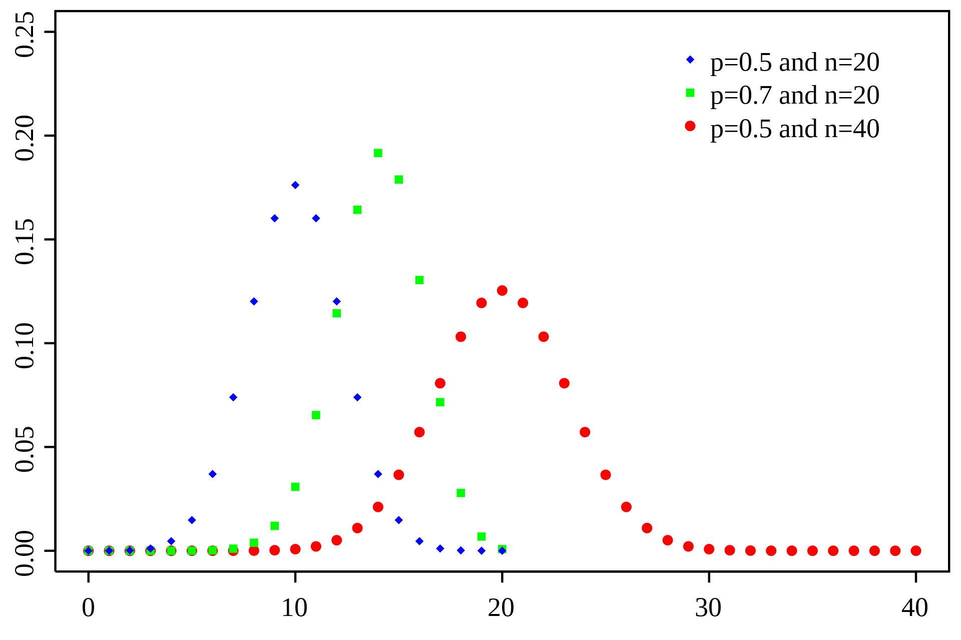
Let randome variable X donates the number of success we achieved in n independent bernoulli trials. Each trail has a same probability p of success. The parameters of a Binomial Distribution includes n and p

Formulation

The PDF of a binomial distribution: \[ f_X(X = k,n,p) = \frac{n!}{k!(n-k)!}p^k(1-p)^{n-k} \] where k = 0,1,2...n

The CDF of a binomial distribution: \[ F(k,n,p) = P(X\le k) = \sum_{i=0}^k \tbinom{n}{i}p^i(1-p)^{k-i} \] The expectation of a binomial distribution is: \[ E[X] = np \]

The variance of a binomial distribution is: \[ Var[X] = np(1-p) \] Properties

• if \(X \sim bin( n, p), Y \sim bin(m,p)\), then \(X+Y \sim bin(n+m,p)\)
• If p is small, \(Bin(n,p)\) is approximately \(Pois(\lambda = np)\) when \(n \to \infty\)
• if n is large and p is not near 0 and 1, \(Bin(n,p)\) is approximately \(N(np, np(1-p))\)

2.3 Geometric Distribution

Story

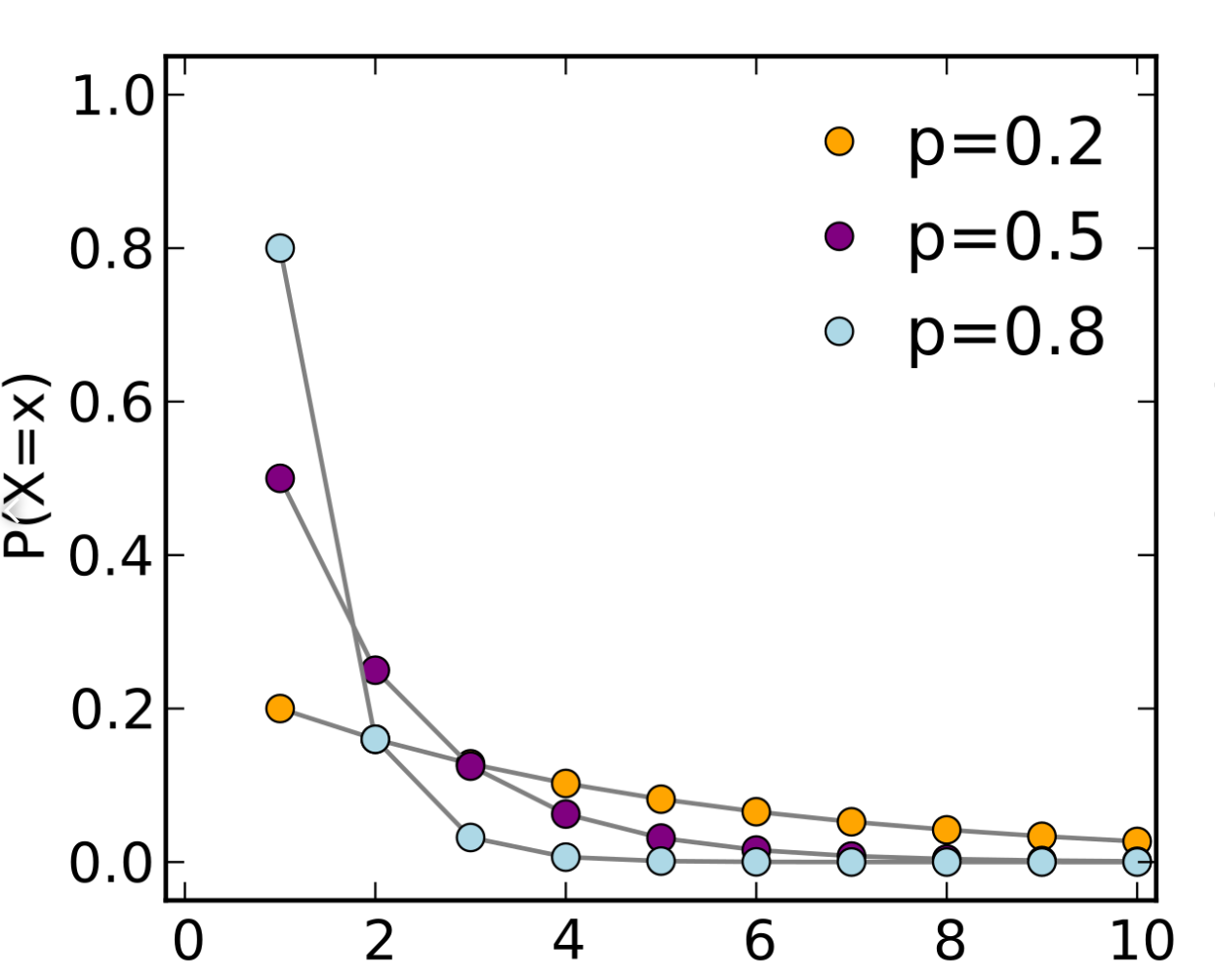
A Geometric Distribution basically have same story like a binomial distribution, except now the X donates times of trails to observe the first success. The only parameter of a Geometric Distribution is p.

Formulation

The PDF of a Geometric Distribution: \[ f(X=k) = (1-p)^{k-1}p \] The CDF of a Geometric Distribution: \[ F(X =k) = 1-(1-p)^k \] The expectation of a Geometric Distribution is: \[ E[X] = \frac{1}{p} \]

The variance of a Geometric Distribution is: \[ Var[X] = \frac{1-p}{p^2} \] Properties

• Memoryless: if \(x \sim Geom(p)\), then \(P(T>t+s|T>t) = P(T>s)\). This suggests no matter how many previous failures happened, the additional number of times of trail needed to observe a success still follows a \(\sim Geom(p)\)

2.4 Possion Distribution

Story

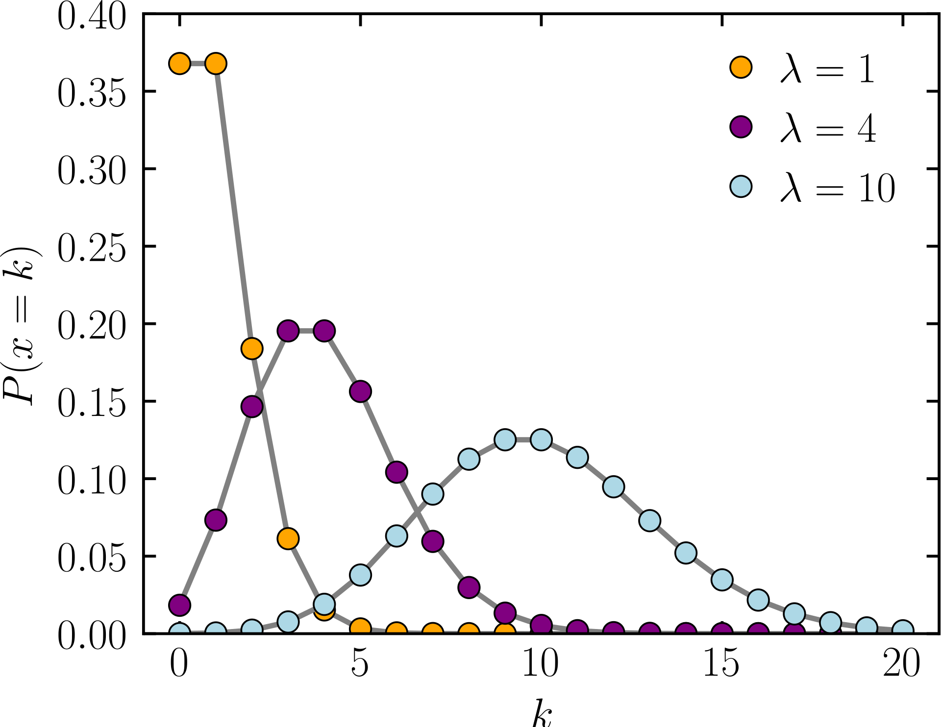
Suppose an event(X = x) happens with a certain probability(usually low probability), let X be the times that event happens in a unit time, then X follows a Possion Distribution. \(\lambda\) is the only parameter for a Possion Distrbution, which is the expectation of X.

Formulation

The PDF of a Possion Distribution: \[ f_X(X = k,\lambda) = \frac{e^ {-\lambda}\lambda^k}{k!} \] where k = 0,1,2...\(\infty\)

The CDF of a Poission distribution: \[ F_X(X=k, \lambda) = e^{-\lambda}\sum_i^k\frac{\lambda^i}{i!} \]

The expectation of a poisson function is: \[ E[X] = \lambda \]

The variance of a poisson function is: \[ Var[X] = \lambda \]

Properties

• Let N(t) denote the number on occurrence of the event in a time t instead of a unit time, it can be proved that \(P(N(t) = n) \sim Pois(\lambda t)\)

• Consider a Poisson Process with rate \(\lambda\), let \(T_n\) denote the time interval between the \(n-1^{th}\) and \(n^{th}\) occurrence of the event, then \(T_1,T_2,..T_n\) is i.i.d. exponential random variable with rate \(\lambda\)

• if \(X \sim pois(\lambda_1), Y \sim pois(\lambda_2)\), then \(X+Y \sim pois(\lambda_1+\lambda_2)\). Oppositely, if a Poisson Process's result can be further classified with n category with probability \(p_1,p_2,..p_n\), where \(\sum_i^np_i = 1\), then we can treat the original poisson process as n sub poisson processes with rate \(\lambda p_1, \lambda p_2,...\lambda p_n\)

• Consider 2 poisson process with rate \(\lambda_1\) and \(\lambda_2\), let \(S_n^1\) denote the time of \(n^{th}\) event of the first process,and \(S_m^2\) the time of the \(m^{th}\) event of the second process: \[ P(S_n^1 < S_m^2) = \sum^{n+m-1}_{k=n} {n \choose m}(\frac{\lambda_1}{\lambda_1+\lambda_2})^k(\frac{\lambda_2}{\lambda_1+\lambda_2})^{n+m-1-k} \]

• Let \(X,Y\) be poisson random variable with rate \(\lambda_1,\lambda_2\), \(X|(X+Y=n) \sim Bin(n,\frac{\lambda_1}{\lambda_1+\lambda_2})\)

3. Continuous Distribution

3.1 Uniform Distribution

Story

The Uniform Distribution, as the name suggests, refers to a probability distribution where all outcomes in a range are equally likely.A uniform distribution has two parameters \(a ,b\), respectively represents the beginning and end of the range of possible outcome

Formulation

The PDF of a uniform distribution: \[ f(x) = \left \{ \begin{aligned} &\frac{1}{b-a} \qquad& for \ a \le x \le b \\ & 0 & elsewhere \end{aligned} \right. \] The CDF of a uniform distribution: \[ F(x) = \left \{ \begin{aligned} & 0 & x < a\\ &\frac{x-a}{b-a} \qquad& for \ a \le x \le b \\ & 1 & x > b \end{aligned} \right. \] The expectation of a uniform distribution: \[ E[X] = \frac{a+b}{2} \] The variance a uniform distribution: \[ V[X] = \frac{(b-a)^2}{12} \]

3.1 Normal Distribution

Story

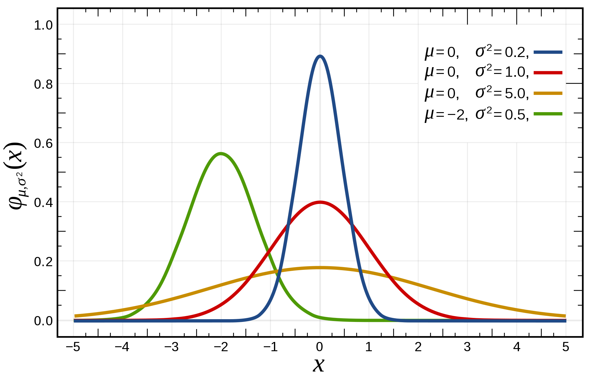
If how the certain value of a continuous random variable X is unknown, we can assume it follows a normal distribution. The parameters of a normal distribution include \(\mu\) and \(\sigma^2\)

Formulation

The PDF of a normal distribution: \[ f(x) = \frac{1}{\sigma\sqrt{2\pi}}e^{-\frac{(x-\mu)^2}{2\sigma^2}} \] A normal distribution does not have a closed-form CDF. It is usually obtained by simulation and approximation. Specifically, we call the denote of a \(N(0,1)\) as \(\Phi\). In real application, we can search the table for the exact value.

The expectation of a normal distribution is: \[ E[X] = \mu \]

The variance of a normal distribution is: \[ Var[X] = \sigma^2 \] Properties

• if \(X \sim N(\mu_1,\sigma_1^2), Y \sim N(\mu_2,\sigma_2^2)\), then \(X+Y \sim N(\mu_1+\mu_2,\sigma_1^2 + \sigma_2^2)\)
• if \(X \sim N(\mu_1,\sigma_1^2)\), then $aX+b N(a+ b, (a)^2) $
• if \(X_1,X_2,..X_n\) all follows normal distribution, than \(X_1^2+X_2^2+...X_n^2\) follows \(\chi^2(n)\)
• For 2 normal distributed variable, it is equivalent to claim that they are uncorrelated(\(E[X_1X_2] = E[X_1]E[X_2]\)) and that they are independent(\(P(X_1,X_ 2) = P( X_ 1)P( X_ 2)\))

3.2 Exponential Distribution

Story

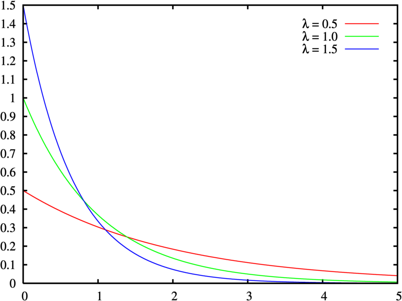
The Exponential Distribution describe same story as poisson distribution, exception the random variable X now donates the time interval between two occurrence of the events. The only parameter for exponential distribution is \(\beta\), where \(\beta = \frac{1}{\lambda}\), representing the probability of occurrence of the event in a unit time.

Formulation

The PDF of an exponential distribution: \[ f(x) = \left\{ \begin{array}{lr} \lambda e^{-\lambda x} & x \ge 0 \\ 0 & x<0\\ \end{array} \right. \]

The CDF of an exponential distribution: \[ F(x) = \left\{ \begin{array}{lr} 1 - e^{-\lambda x} & x \ge 0 \\ 0 & x<0\\ \end{array} \right. \] The expectation of an exponential distribution is: \[ E[X] = {1\over \lambda } \]

The variance of an exponential distribution is: \[ Var[X] = {1\over \lambda^2} \] Properties

• Memoryless: if \(x \sim Expo(\beta)\), then: \[ P(T>t+s|T>t) = P(T>s) \] That is given the information of the state of the current moment, the additional time for the random event is still a \(Expo(\beta)\)

• If \(X_1,...,X_n\) are independent exponential random variables with common rate λ, then \(\sum_i^nX_i\) is a $(n, λ) $random variable. If they instead follow exponential distribution with different rate \(\lambda_1,\lambda_2,...\lambda_n\), then: \[ P(\sum_i^nX_i) = \sum_i^nC_{i,n}\lambda_ie^{-\lambda_it} \] Where: \[ C_{i,j} = \prod_{j\ne i} \frac{\lambda_i}{\lambda_j-\lambda_i} \]

• Let \(X_1,X_2,...X_n\) be exponentially distributed random variable with rate \(\lambda_1, \lambda_2,...\lambda_n\), then: \[ P(min(X_1,X_2,...X_n) = X_i) = \frac{\lambda_i}{\sum_i^n\lambda_n} \]

• if we have independent \(X_i \sim Expo( \lambda_ i)\), then: \[ \begin{aligned} min(X_1,X_2,..X_k) &\sim Expo(\lambda_1+\lambda_2+...+\lambda_k) \\ max(X_1,X_2,..X_k) &\sim Expo(\lambda)+Expo(2\lambda)+...+Expo(k\lambda) \end{aligned} \]

• if \(X \sim Expo(\lambda)\), then \(C*X \sim Expo({\lambda \over C})\)

3.3 Gamma Distribution

Story

Suppose in the exponential distribution scenario, you want to observe the event for \(\alpha\) times before you stop, then the time you need to do that would follows a Gamma distribution

Formulation

The PDF of a Gamma distribution: \[ f(x) = \frac{x^{\alpha-1}\lambda^\alpha e^{-\lambda x}}{\Gamma(\alpha) } \]

\[ \Gamma(\alpha) = (\alpha-1)! \qquad \alpha \ is \ Z \]

\[ \Gamma(\alpha) = (\alpha-1)\Gamma(\alpha-1) \qquad \alpha \ is \ R \]

\[ \Gamma(\frac{1}{2}) = \sqrt{\pi} \]

The PDF of a Gamma distribution: \[ F(X)= \frac{\gamma(\alpha,\beta x)}{\Gamma(\alpha)} \] where \(\gamma(\alpha,\beta x)\) is a lower incomplete gamma function: \[ \gamma(s,x) = \int_0^x t^{s-1}e^{-t}dt \] The expectation of a gamma distribution is: \[ E[X] = \alpha \beta \]

The variance of a gamma distribution is: \[ Var[X] = \alpha \beta^2 \] properties

• if \(X \sim \Gamma(\alpha_1,\beta), Y \sim \Gamma(\alpha_2,\beta)\), then \(X+Y \sim \Gamma(\alpha_1+\alpha_2, \beta)\)

• When \(\alpha = 1\), a gamma distribution is equivalent to a exponential distribution

3.4 Beta Distribution

Story

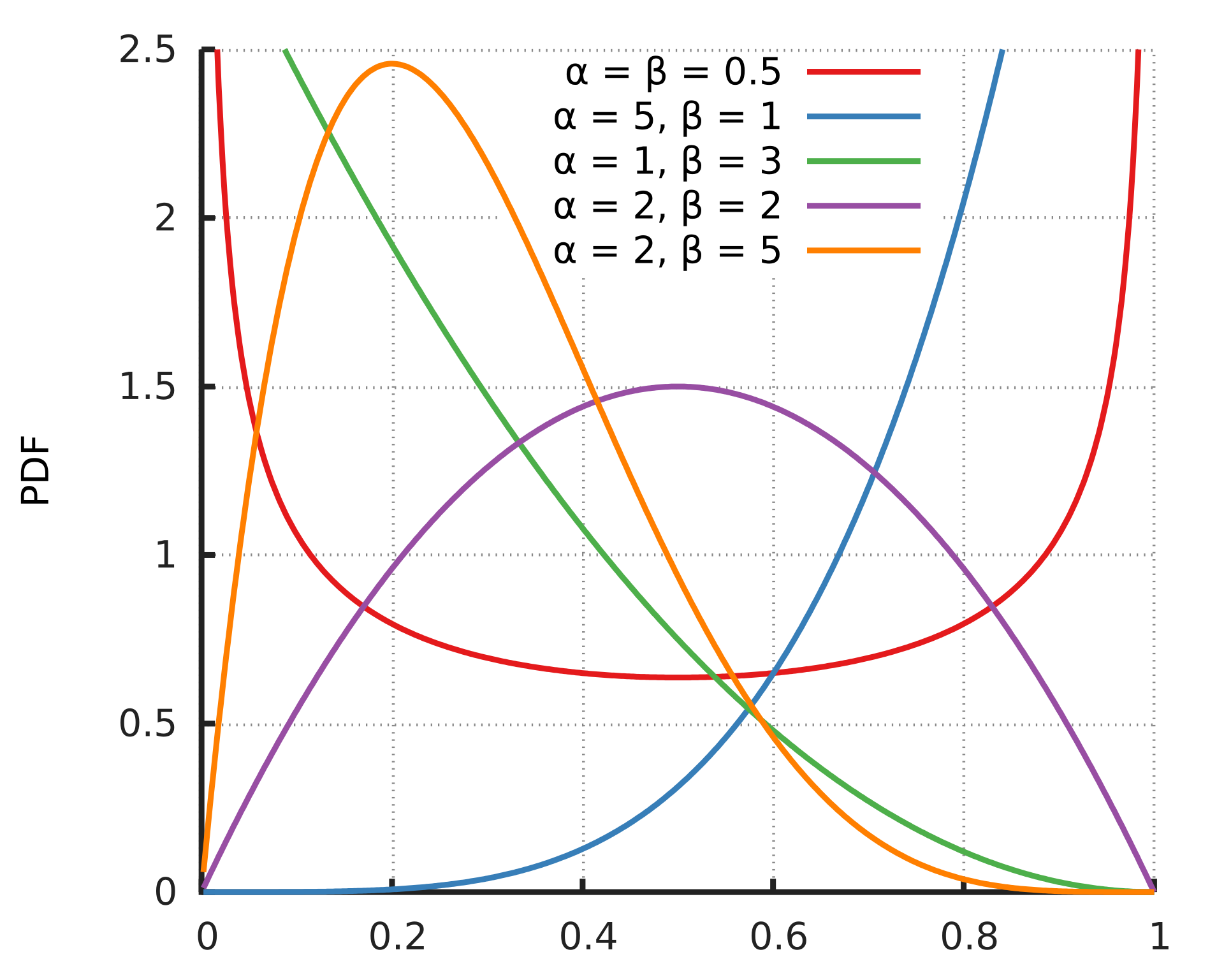
The beta distribution is the conjugate prior distribution of a binomial distribution in a Bayesian Inference Context. Thus, it can be interpreted as the PDF of the parameter of a binomial distribution, which is the probability to success in the trail. In other world, it is a likelihood function.

Formulation

The PDF of a beta distribution: \[ f(x) = \frac{1}{B(\alpha,\beta)}x^{\alpha-1}(1-x)^{\beta-1} \] where:

• \(\alpha\) is the number of observations of success

• \(\beta\) is the number of observations of failure

• \(B(\alpha, \beta)\) is a standard B function. It is applied to make the integrate of the PDF one \[ B(\alpha,\beta) = \frac{\Gamma(\alpha+\beta)}{\Gamma(\alpha)\Gamma(\beta)} \]

The CDF of a beta distribution: \[ F(x;\alpha,\beta) = \frac{B_x(\alpha,\beta)}{B(\alpha,\beta)} \]

where \(B_x(\alpha,\beta)\) is a incomplete beta function: \[ B_x(\alpha,\beta) = \int_0^x t^{\alpha - 1}(1-t)^{\beta-1} dt \] The expectation of a beta distribution is: \[ E[X] = \frac{\alpha}{\alpha + \beta} \]

The variance of a gamma distribution is: \[ Var[X] = \frac{\alpha \beta}{(\alpha+\beta)^2(\alpha+\beta+1)} \] Properties

• if \(X \sim \Gamma(a,\lambda), Y \sim \Gamma(b,\lambda)\), X and Y are independent, then \(\frac{X}{X+Y} \sim B(a,b)\)

• After n trial, if x success is observed, the distribution of p is updated to \(B(\alpha+x,\beta+n-x)\)

3.5 \(\chi^2\) Distribution

Story

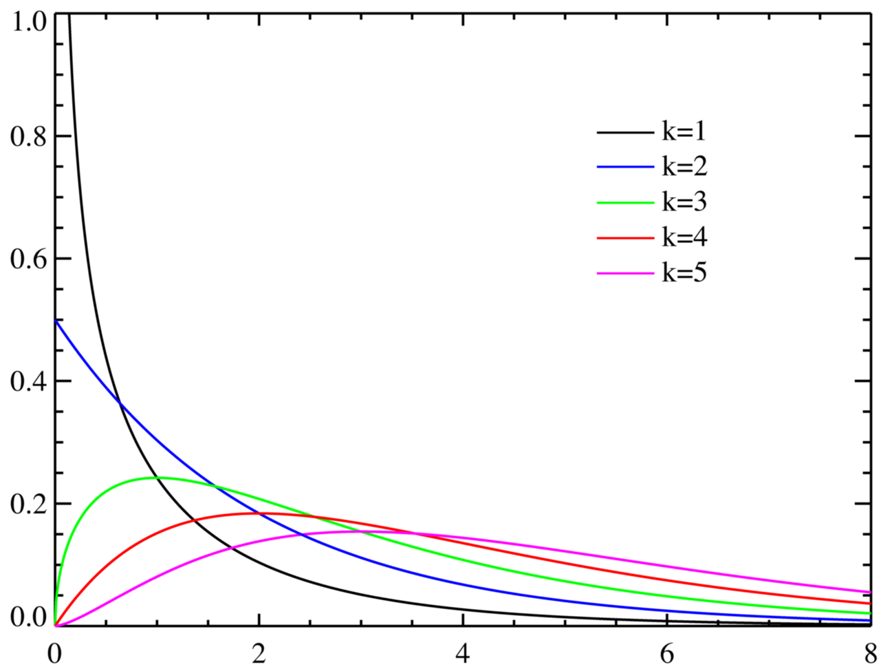
Suppose k independent random variable \(Z_1,..Z_ k\) all follow standard normal distribution, then define random variable X as \(\sum_iZ_i^2\), then X follows a \(\chi^2\) distribution. k is the only parameter of \(\chi^2\) distribution, representing the number of independent variable(degree of freedom)

Formulation

The PDF of a \(\chi^2\) distribution: \[ f(x) = \frac{1}{2^{\frac{k}{2}}\Gamma(\frac{k}{2})}x^{\frac{k}{2}-1}e^{\frac{-x}{2}} \] The CDF of a \(\chi^2\) distribution: \[ F_k(X)= \frac{\gamma({k \over 2},{x \over 2})}{\Gamma({k \over 2})} \]

The expectation of a \(\chi^2\) distribution is: \[ E[X] = k \]

The variance of a \(\chi^2\) distribution is: \[ Var[X] = 2k \] Properties:

• If \(\chi^2(k_1)\) and \(\chi^2(k_2)\) are independent, then \(\chi^2(k_1) + \chi^2(k_2) \sim \chi^2(k_1+k_2)\)

• When k is large, a \(\chi^2\) distribution is similar to a normal distribution

4. Multivariate Distribution

A Multivariate Distribution is the joint PDF of a vector of variables

4.1 Multinomial Distribution

Suppose there are n items fall into k buckets, where the probabilities each items fall into the k buckets is \(\vec{p} = (p_1,p_2,...p_k)\), let \(X_i\) donates the number of items fall into the \(i^th\) bucket, then a vector \(\vec{X} = (X_1,X_2,...X_k)\) follows a Multinomial Distribution MulNm(n,\(\vec{p}\) )

The Joint PDF of a Multinomial Distribution is: \[ P(\vec{X} = \vec{n})=\frac{n!}{n_1!n_2!...n_k!}p_1^{n_1}p_2^{n_2}...p_ k^ {n_k} \] where \(\vec{n}\) is a specifc combination of numbers of items fall into each buckets:\(\vec{n} = (n_1,n_2...n_k)\), and $n_ 1+n _2+...+n_k = n $

The Expectation Vector \(\vec{ E }\) would be \((np_1,np_2,...np_k)\)

The Variance vector \(\vec{ V }\) would be \((np_1(1-p_ 1),np_2(1-p_2),...np_k(1-p_k))\)

The Covariance for \(X_i\) and \(X_j\) would be \(Cov(X_i,X_j) = -np_ip_j\)

4.2 Multivariate Normal Distribution

For a vector \(\vec{X} = (X_1,X_2,...X_k)\) , if every linear combination of this vector is normally distributed, then \(\vec{ X }\) follows a Multivariate Normal Distribution MulNorm(\(\vec{\mu},\vec{\sigma^2}\)).

The Joint PDF of a MVN Distribution is: \[ f(\vec{X}) = \frac{1}{\sqrt{(2\pi)^k|\Sigma|}} e^{-\frac{1}{2}(X-\mu)^T\Sigma(X-\mu)} \] Where \(|\Sigma|\) is the determinant of the Covariance Matrix

The Covariance for \(X_i\) and \(X_ j\) is calculated by: \[ Cov(X_i,X_j) = E[(X_i-\mu_{X_i})(X_ j- \mu_{X_j})] = E[X_iX_j]-E[X_i]E[X_j] \]

5. Distribution Transformation

Suppose the PDF of a random variable x is \(f_X(x)\), define \(y = t(x)\), then: \[ x = t^-{1}(y) \] let the CDF of X and Y be \(F_X,F_Y\) \[ P(Y<y) = P(X<x) \]

\[ F_Y(y) = F_X(t^{-1}(y)) \]

\[ f_Y(y) = F'_Y(y) = (t^{-1}(y))'f_X(t^{-1}(y)) \]

With Such rules , let \(Y = F(X)\) \[ f_Y(y) = (F^{-1}(y))'f_X(F^{-1}(y)) = F(F^{-1}(y))'F^{-1}(y) = F(F^{-1}(y))' = y' = 1 \] Thus, if a randam variable \(u = CDF(X)\), then $u U(0,1) $

From	Transformation	to
\(Expo(\lambda)\)	\(Y = 1-e^{-\lambda x}\)	U(0,1)
U(0,1)	\(Y=\sqrt{2}h^{-1}(2X-1)\), \(h(x) = \frac{2}{\sqrt{\pi}}\int_0^xe^{-t^ 2}dt\)	N(0,1)

In many applications, we want to transform a non-normal distribution into a normal one. We know that a normal distribution does not have a closed-form CDF, we need to approximate it through error function h(x). In some case, we use a transformation to directly let \(f_Y(y)\) have an approximate formulation as the target distribution. Then we define an error function to measure the loss of y and E[y] under target distribution, and train the parameters of the tranformation.

From	Transformation	to
\(Expo(\lambda)\)	\(Y =\frac{X^\theta-1}{\theta}\)	\(N(\mu,\sigma^2)\)
\(Expo(\lambda)\)	\(Y=log_\theta（1+X）\)	\(N(\mu,\sigma^2)\)

There are many improved transformation algorithm like Box-cox, Yeo-johnson and Box-Muller. For more transformation methods for data distribution in machine learning, refer to this article.

A: Distribution Type and their properties