Normality Test and Distribution Type Transformation

1. Normality and Distribution Type Transformation

In feature engineering, sometimes we need to transform the distribution type to make the data fit the model. In most scenarios, we want to transform a non-normal distributed variable into a normal distributed variable.

2. Normality Test

Before transformation, we need first to examine the normality of the data to decide which features to transform.

2.1 Visualized Method

Histogram

The histogram is one of the simplest method to test normality. If the histogram are bimodal cureve or a trailing curve, then there is a normality problem

P-P Plot and Q-Q Plot

P-P plot use the cumulative frequency of the sample as a X -axis, the cumulative probability of the variable under a normal distribution assumption as a Y-axis

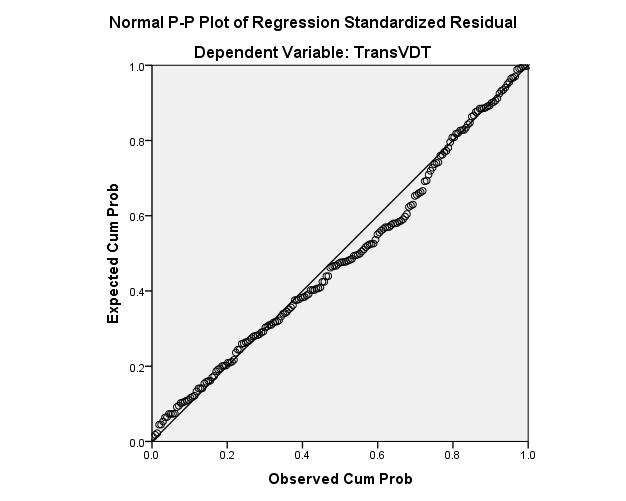
If the points in the graph are approximately around a line from (0,0) to (1,1), then sample reflect a normal distribution. Otherwise, there is a normality problem

The Q-Q Plot is a variant of P-P Plot. The only difference is the axis is now the quantile instead of the cumulative probability.

2.2 Hypothesis Testing Method

Skewness and Kurtosis

Skewness and Kurtosis are both statistics.

Skewness is the standardized 3rd central moment of the sample: \[ S = \frac{1}{n-1}\sum_{i=1}^n(x_i-\bar{x}^3)/s^3 \] The kurtosis is the standardized 4rd central moment. In calculation we usually minus 3 to let the kurtosis of normal distribution be 0 \[ K = \frac{1}{n-1}\frac{\sum_{i=1}^n(x_i-\bar{x}^4)}{s^4}-3 \] where s is the standard deviation

When the variable folllows a normal distribution, both statistics should be 0. Thus we can use a hypothesis testing on these two parameters two decide normality. Let \(SE_S, SE_K\) denote the standard error: \[ SE_S = \frac{6N(N-1)}{(N-2)(N+1)(N+3)} \]

\[ SE_K = \frac{4(N^2-1)SE_s}{(N-3)(N+5)} \]

Construct Z score :\(Z_S = \frac{S}{SE_s}, Z_K = \frac{K}{SE_K}\). Given \(\alpha\) and \(\beta\), we can do a Z test to decide normality.

A improved version of testing based on Skewness and Kurtosis is D'Agostino's K-squared test, which construct a \(\chi^2\) test statistics by combining skewness and kurtosi. It is a common and powerful method for normality test.

K-S Testing

Kolmogorov–Smirnov test is method to test if a empiric distribution is different from a theoretical distribution. In other word, if the variable distributed as we want.

Let \(F_n,F_0\) respectively represent the CDF of the empiric distribution and the theoretical distribution. n is the sample size. Construct test statistics as \[ D_n = sup_x \ |F_n(x) - F_0(x)| \] where sup represent the supremum. If \(F_n = F_0\) , the limit of \(D_n\) should be zero. Given significance level \(\alpha\), find \(t_\alpha\) such that \(P( \sqrt{n}D_n \ge t_\alpha) = \alpha\), the rejection area then would be \([\frac{t_\alpha}{\sqrt{n}},+\infty)\)

In normality test, we can use K-S test to decided whether the variable follows a normal distribution by replacing supreme with maximum. \(F_n,F_0\) would be the observed cumulative frequency of sample and cumulatively probability under normal distribution assumption

\(\chi^2\) Test for fitness

The \(\chi^2\) Test for fitness works similarly like the K-S test in normality test. Construct the \(\chi^2\) test statistics with observed cumulative frequency of sample and cumulatively probability. \(\chi^2\) Test for fitness is easier when the test statistics are discrete. For continuous variable, we need to discretize the variable

3. Distribution Type Transformation

3.1 Monte Carlo Integral

A theoretical method to inverse the CDF of the variable and transform the distribution into a normal distribution, for specific details, refer to this article

Box-Muller

A simpler way to obtain normal-distributed vairable from uniformly distributed variable is the Box-Muller. Given two uniformly distributed variables \(U_1, U_2\): \[ Z_1 = \sqrt{-2lnU_1}cos(2\pi U2) \]

\[ Z_2 \ \sqrt{-2 lnU1} sin(2\pi U2) \]

It can be proved that \(Z_1, Z_2 \sim N(0,1)\). Through this method, we can transform pairwise variable without knowing the error function of the single variable. However, the CDF of both variables should still be known.

In real application, it is difficult to obtain the accurate cumulative density function. Thus, MC method only works well when the CDF of the variable is given in a closed form. In most scenarios, we would use other transformation to approximate a normal distribution

3.2 Log Transformation

We can try to approximate normal distribution through log transformation: \[ X' = log_a(X+k) \] Where a and k are parameterswe can adjust. Greater a has stronger power to correct skewness. Usually we would try \([e, 10]\). K is a positive correction term ensuring there's no negative, zerr or extreme small values in the data.

3.3 Power Transformation

We can try to approximate normal distribution through power transformation: \[ X' = X^a \] when the vairable is a ratio, we can also add a arcsin transformation: \[ X' = arcsin(X^a) \] Improved power transformer includes:

Box-Cox \[ X' = \left\{ \begin{aligned} \frac{X^\lambda-1}{\lambda} \qquad& \lambda \ne0\\ ln(X) \qquad & \lambda = 0 \\ \end{aligned} \right. \] Yeo-Johnson

\[ X' = \left\{ \begin{aligned} &\frac{(X+1)^\lambda-1}{\lambda} \qquad& \lambda \ne0, X\ge 0\\ &ln(X)+1 \qquad & \lambda = 0, X \ge 0\\ &\frac{-[(-X+1)^{2-\lambda}-1]}{2-\lambda} \qquad& \lambda \ne 2, X<0\\ &-ln(-X+1) \qquad&\lambda=2, X<0 \end{aligned} \right. \] where\(\lambda\) is a parameter that can be optimized through Maximum Likelihood Estimation(MLE). The Box-Cox transformer requires X to be strictly positive, while the Yeo-Johnson transformer can accept any numbers.