Outlier Detection in Feature Engineering
Outlier Detection and Processing
1. About Outlier
What is an outlier
In statistics, an outlier is a data point that significantly differs from other observations.
Why we need outlier detection?
Outliers can lead to bias in machine learning. Many models, especially those have strong hypothesis on data distribution(LR,K- Means) would be influenced, or even be unable to converge if outliers exist in training data. Some business and engineering problem, like fraud detection and quality control, are also a outlier detection problem in nature. For this article, we only look to the outlier detection for feature engineering.
2. Statistical Method
2.1 One-dimension Method
2.1.1 Six \(\sigma\) Method
Given a one-dimension variable X that satisfies Gaussian Distribution: \(X~N(\mu,\sigma)\), where \(\mu\) and \(\sigma\) is the mean and standard error of the sample:
If a point \(x \notin (\mu-3\sigma,\mu+3\sigma)\), then x can be flagged as an outlier
2.1.2 Grubb's Test
Grubbs' Test is a kind of hypothesis testing that based ib the following hypothesis:
\(H_0\): There are no outlier in the observations
\(H_1\): There are only one outlier in the observations
There are several constraints for Grubb's Test:
- The Grubb's test can detect one outlier in a single test. If we want to test all data point, we can replace G statistics with z-score to test all samples. If we belive there are a large number of outliers exsits, we should consider other method.
- To apply G test, the variable must follow a Gaussian Distribution
- The test variable must be univariate, if we want to apply the test on multivariate vector, we can calculate the distance between \(x_i\) and \(\bar{x}\), and use the distance d as the test variable
Define statistics G as: \[ G = \frac{\max|X_i - \bar{X}|}{s} \] which is the z-score of the farthest data point
If: \[ G > \frac{N- 1}{\sqrt{N}}\sqrt{\frac{t_{\frac{\alpha}{2N},N-2}^2}{N-2+t_{\frac{\alpha}{2N},N-2}^2}} \]
Where:
- N is the sample size
- t represents the t score, suppose the orignal dataset can be trasformed to a t distribution
- \(\frac{\alpha}{2N}\) is the significance level (If it's a single-side test, then \(\frac{\alpha}{N}\))
- N-2 is the degree of freedom
Then maxnium/minimum of these data points can be flagged as an outlier
2.1.3 BoxPlot
Boxplot is depicted as follows:
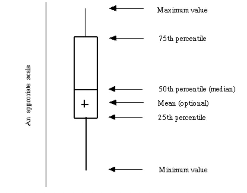
It shows the maximun, 75 percentile, median, 25 percentile and minimum of a dataset.
Note that the maxinum and minimum are not the original values of the data, instead it's calculated as: \[ Max = \min(M,Q_3+1.5IQR ) \]
\[ Min = \max(m,Q1-1.5IQR) \]
where:
- M,m is the actual maximum, minimum of the dataset
- Q1,Q3 is the 25,75 percentile of the dataset
- IQR is the intermediate quantiles range of the data, \(IQR = Q3-Q1\), which is the length of the box
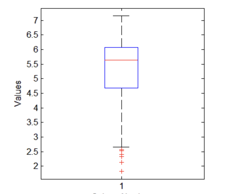
- if the actual maximum is smaller than the calculated maximum, then plot with the actual maximun, and there are no outliers. The same apply to minimun
- The data points outside the range of calculated minimum and maximum would be labeled as outliers
2.2 High-dimension method
2.2.1 \(\chi^2\) Test
[ongoing]
2.2.2 Gaussian Distribution Detection
The P value for a high-dimenstion data point is quiet difficult to calculate. We can instead set a threshold \(\epsilon\), suppose a data set \(D = \{ x^{(i)} : 0\le i \le m \}\) ,let \[ \mu = \frac{1}{m}\sum_i^m x^{(i)},\sum=\frac{1}{m}\sum(x^{(i)}-\mu)(x^{(i)}-\mu)^T \]
\[ p(x) = \frac{1}{2\pi^\frac{n}{2}|\sum|^\frac{1}{2}}exp(-\frac{1}{2}(x-\mu)^T\Sigma^{-1}(x-\mu)) \]
if \(p(x) < \epsilon\), the data point can be regard as an outlier
3. Distance-based Method
For details of distance metrics, refer to this article
3.1 Angle-based Method
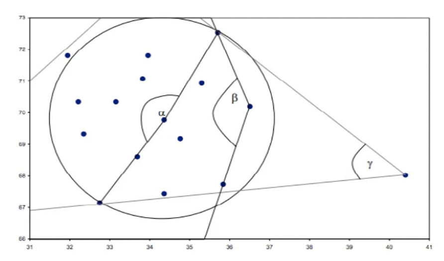
From this graph it is obvious to discover that the inner angle consists of an outlier and any two other points have almost same size. Thus we can define the Angle-based outlier factor as: \[ ABOF(o) = VAR_{x, y \ne o}[\frac{\vec{ox}\cdot \vec{oy}}{dist(o,x)^2dist(o,y)^2}] \] where:
- o is any points in the dataset
- x, y is all other point in the dataset
- dist is the distance metirc, usually euclidean distance
THe ABOF of an point is the variance of the consine of it and all data pairs consists of other data points. The smaller ABOF a data point has, the more likely it would be an outlier
The complexity of ABOF is \(O(n^ 3)\). Besides, when applying euclidean distance, the scale of data would have an effect
3.2 Nearest Neighbor Method
The steps of Nearest neighbor method is given as follow
- Calculate the KNN of a data point
- Add up the distances of the KNN
- Repeat for every points and sort the sum of distance in descending order
- The points with larger sum of distance is more likely to be outliers
The tranditional KNN is not suitable for sparse dataset. To improve this, we can apply the following metrics to make judgement:
Local Outlier Factor(LOF) : The ratio of the local average density of the KNN of the data point and the local average density of the point itself, the greater LOF a point has, the more likely it would be an outlier
Connectivity Oulier Factor(COF) : Outlier are points p where average chaining distance of p is higer than average chaining distanc of p's neighbors. Points with higher COF has sparser surrounding than its neighbors
3.3 Distance-based Test
As mentioned in 2.1.2, for high dimension data, we can apply tests on the distance of X and \(\bar{X}\) instead of the original vector.
4. Model-based Method
4.1 Clustering Model
Clustering model can be used as outlier detection methods.
- For distance-based clustering, like K-Means, outliers are points have largest distance to their cluster centroids
- For density-based clustering, like DB-SCAN, outliers would be labeled by the model
For details of clustering algorithm, refer to ongoing
4.2 One-class SVM
4.3 Isolation Forest
4.4 PCA
PCA can also be utilized as an outlier detection method. In PCA, we would decompose the covariance matrix, the \(m^{th}\) eigenvector \(\vec{e_m}\) represent present the direction of the \(m^{th}\) principle component, and the eigenvalue \(\lambda_m\) is the variance on that direction, which also indicates the importance of principal component. Therefore, \(\vec{x}\cdot \vec{e_m}\) represents mapping all original features to the direction of \(m^{th}\) principal component and adding up all decomposed vectors on that direction, as \(\vec{x}\) is standardized.
Thus, we can define the deviation extent of an sample on a certain principle component direction: \[ d_m = \frac{\vec{x_i}\cdot \vec{e_m}}{\lambda_m} \] The role of \(\lambda\) is to make deviation extent more comparable, as the size of variance can be different to some degree.
With such definition, we might discover the deviation extent of an outlier could probably larger on each direction are generally higer, as shown below:
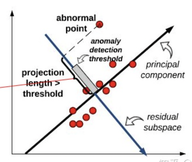
we can define the Anomaly score of a data point as: \[ Score(x_i) = \sum_m d_m \] The higher this score is, the more likely a data point would be an outlier.
This score is equalvalent to the Mahalanobis Distance between the data sample and the mean, as the M distance is the euclidean distance in standard principal components space: \[ D = \sqrt{(X-\mu)^TS^{-1}(X-\mu)}=\sqrt{X^TE\lambda^{-1}E^{-1}X} = \sqrt{\frac{(EX)^2}{\lambda}} = \sqrt{d} \] In this equation:
- X is standardized vector, \(\mu\) is thus 0
- \(S^{-1}\) is the inverse of the covariance matrix
- \(\lambda\) is the eigenvalues matrix, which is a diagnal matrix, \(\lambda^{-1} = \frac{1}{\lambda}\)
- E is the eigenvalues matrix, which is a orthonormal matrix, \(E^{-1} = E^T\)