Common Loss Function in Machine Learning

1.Numerical Output

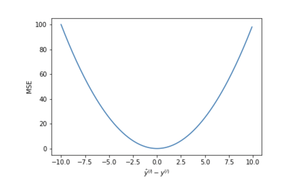
1.1 MSE(L2 Loss)/RMSE

Mean Squared Error(MSE) \[ MSE = \frac{1}{n}\sum_i^n(y_i-\hat{y})^2 \]

• MSE is differentiable any where, which makes it suitable for gradient descent optimizer
• With gradient decrease, the MSE will decrease, which means MSE is effective with fixed learning rate
• The squared operator gives enlarge the loss, thus MSE is sensitive ti outlier, if outlier is meant to be detected, suing MSE is fine. If the outlier is treat as part of the training data, MSE is not an ideal loss function (e. g. prediction model for sales promotion day)

Root Mean Squared Error(RMSE)

RMSE is the square root of MSE \[ RMSE = \sqrt{MSE} \]

• RMSE is on the same scale with MSE, but it make the loss more interpretable in some case(e.g prediction on product price)

Mean Squared Log Error(MSLE) \[ MSLE = \frac{1}{n}\sum_i^n(log(1+y_i)-log(1+\hat{y)}^2 \]

• Add one to avoid the appearance of log 0
• MSLE is ideal when we priorly know there's a exponential relationship between Y and some X(e. g. Population). However, in many cases we would transorm data with exponential distribution in data preprocessing so that the exponential relationship would be eliminated. Thus, MSLE is not frequently used

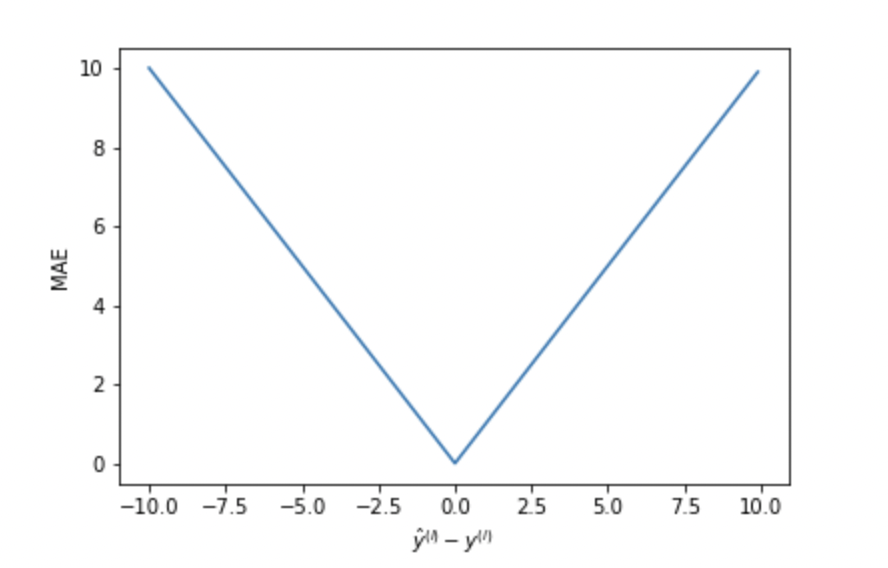
1.2 MAE (L1 Loss)/MAPE

Mean Absolute Error(MAE) \[ MAE = \frac{1}{n}\sum_i^n|y_i-\hat{y}| \]

• MAE is not sensitive to outlier, it is less likely to cause gradient explosion
• The gradient for any loss is the same, which means MAE does not converge well with fix learning rate
• MAE is not differentiable at 0

MAPE

MAPE is the mean percentage absolute error \[ MAPE = \frac{1}{n}\sum_i^n\frac{|y_i-\hat{y}|}{y_ i} \]

• It can more clearly deliver the degree of deviation rather than the scale of the error

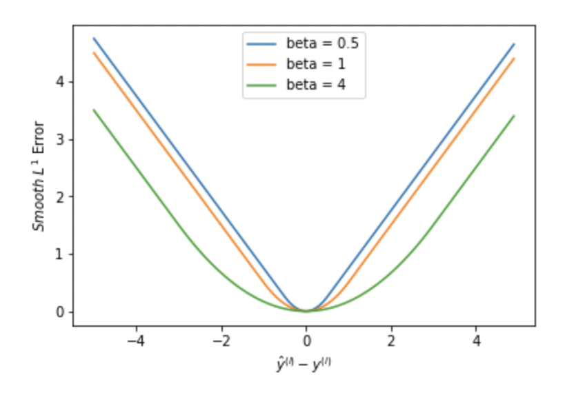
1.3 Smooth L1(Huber Loss)

\[ L = \frac{1}{n}\sum_i^nz_ i \]

\[ z_i = \left\{ \begin{aligned} MSE \qquad& |y -\hat{y}| < \beta \\ MAE \qquad & elsewhere \\ \end{aligned} \right. \]

• \(\beta\) is a defined threshold for error of outlier. If the error is within \(\beta\), apply MSE, otherwise, apply MAE. Huber Loss combines the advantages of L1 and L2 Loss
• Huber loss is ideal for NN

1.4 Log-cosh Loss

\[ L = \sum_ i^ nlog(cosh(y_i-\hat{y_i})) \]

• Log-cosh has almost every virtue of Huber loss, the difference is, it is second-differentiable anywhere, such method is very useful when applying newton-method optimzer
• However, when erro is very big, Log-cosh loss still would have gradient or hessian problem(gradient remains same when loss decrease). Just like MAE

2. Categorical/Probability Output

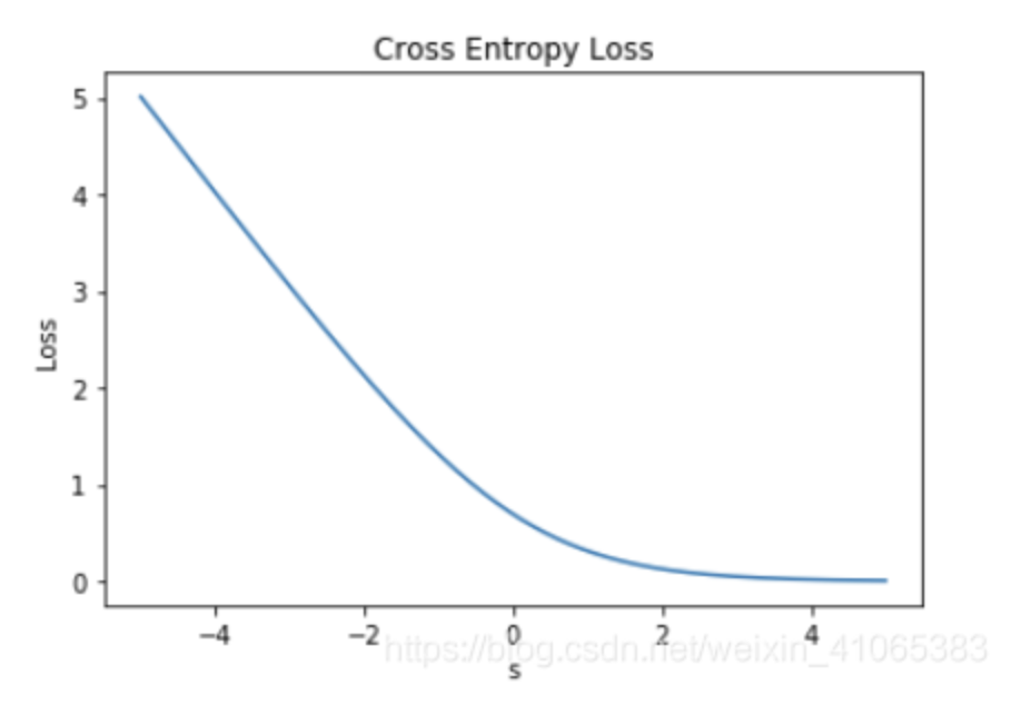
2.1 Log Loss/Cross Entropy Loss

Log Loss is basically the same concept as the cross entropy, the only difference is that it can be applied at a single sample by replaceing true probability p(x) with 1 if \(y_ {true} = m\). The average loss of all sample is the Log Loss or Cross Entropy Loss.

For Cross Entropy, refer to here

When it come to a binary classification scenario, the Log Loss can be written as: \[ LogLoss = -\frac{1}{n}\sum_i^n [y_ilog(p(y_i))+(1-y_i)log(1-p(y_i))] \]

where \(y_i\) is the true value of output and \(p(y_i)\) is the probability predicted by the model.

• The gradient would decrease as Log Loss decrease, thus Log Loss can work with fixed learning rate
• Sentive to outlier
• GDBT usually apply Log Loss as loss function(classification)

The following picture is the log loss of the prediction on a positive sample:

2.2 Exponential Loss

\[ L = \frac{1}{n}\sum_i^ne^{-yf(x)} \]

• Theoretically, the optimal of Exponential Loss and Log Loss is the same(\(\frac{1}{2}log\ odds\)), the advantage of exponential loss is that is is easier to calculate, thus can make optimzer update the weight with less cost
• Sentive to outlier
• AdaBoosting usually apply Exponential Loss as loss function(classification)

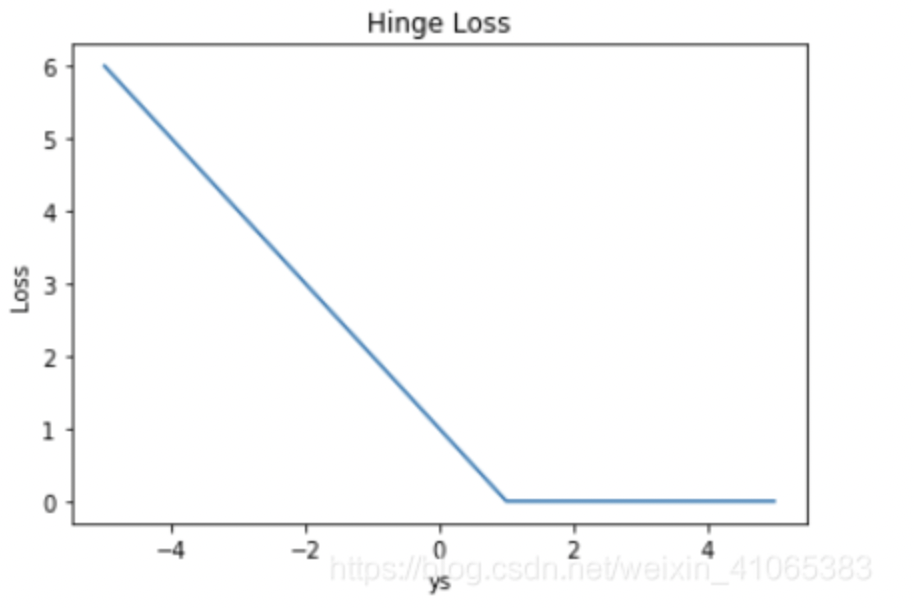
2.3 Hinge Loss

\[ L = \frac{1}{n}\sum_i^n max(0,1-yf(x)) \]

• If the model label the sample correct, the loss is 0
• Less sensitive to outlier
• SVM usually adopt Hinge Loss as loss function

2.4 Focal Loss

Focal Loss is a improved version of Cross Entrophy Loss \[ L_ f = -\frac{1}{n}\sum_i^n\sum_ j^m\alpha_ j(1-p(y ))^\gamma y log(p(y)) \]

• Focal Loss add a focus factor \((1-p(y))\), so that those sample with high predicted probability, which are the ""easy samples", donate less loss. Compare to CE Loss, Focal Loss focus on those "hard samples"
• Focal Loss also add a balance factor(optional), which is the percentage of a certain category of y among all samples. This make focal loss can deal with imbalanced data
• \(\gamma\) is a influence parameter. When \(\gamma = 0\), the Focal Loss become CE Loss. In preactice, we usually set \(\gamma = 2\)

2.5 Impurity

Impurity is a kind of loss functions usually applied in splitting in decision tree

Gini Impurity \[ I_G = 1- \sum_{i}^m P(Y=C_i)^2 \]

• Lower \(I_G\) , better classification performance
• For decision tree model, calculate \(I_G\) for each split and use combined Gini Impurity(\(\sum I_G\)) as loss of the spiltting

Information Gain

For details of Information Gain, refer to here \[ IG = H(Y) - H(Y|X) \] where X is the feature the spliting based on (X>c,X=1)

• IG is the degree that uncertainty reduce after the spilting, the greater IG is, the better a split is
• We can calculate the Information Gain Rate \(IGR = \frac{IG}{H(Y)}\) to present the degress of uncertainty reduction more directly