Evaluation for Regression

Evaluation for Regression Model

1. Evalution for goodness of fitting

1.1 Coefficient of Determination

For a regression model, we believe there's such a equitation: \[ \begin{aligned} TSS &= ESS + RSS\\ \sum_i^n(y_i-\bar{y})^2 & =\sum_i^n(\hat{y_i}-\bar{y})^2+\sum_i^n(y_i-\hat{y_i})^2 \end{aligned} \] In this equations, TSS stands for the total sum of squared error, which is the variance of the output variable. ESS stands for the explained sum of squared error, which represents estimated variance of Y, ot to say, the variance explained by the model. The RSS stands for the residual sum of squared error, which represents the error casued by the model's failure to capture the pattern.

\[ R^2 = \frac{ESS}{TSS} = 1-\frac{RSS}{TSS} \]

• \(R^2\) represent how many variance of Y are interpreted by the model
• If \(R^2 = 0\), TSS = RSS, which means the model equals to a model that simply predicted all samples as the average of Y, which indicates the model has a bad performance. Thus, we want \(R^2\) to approximate 1.
• \(R^2\) is not a true square number, the range of it is \((-\infty,1])\)

1.2 Single Factor Significance Evaluation(t-Test)

For a linear regression model, we can use hypothesis testing to determine whether the effect of the independent variable on the dependent variable is significant. Assuming a relationship between an independent variable \(X_1\) and a dependent variable \(Y\):

\[ Y = \beta_0 + \beta_1X_1+\epsilon \]

According to the Bayesian school, assuming that \(\beta_1\) follows a normal distribution, if the effect of \(X_1\) on \(Y\) is not significant, then the mean of this normal distribution should be very small. Therefore, our null hypothesis is \(H_0: \beta_1 = 0\). By calculating the standard error of \(\beta_1\):

\[ SE(\beta_1) = \sqrt{V[\beta_1]} = \sqrt{\frac{\hat{\sigma^2}}{\sum_i^n(x_{i,1} - \bar{x_1})/n}} \]

where:

\[ \hat{\sigma^2} = \frac{1}{n-2}\sum_i\hat{\epsilon}^2 \approx MSE \]

We can construct the t statistic \(t_{\beta_1} = \frac{\hat{\beta_1}}{SE[\hat{\beta_1}]}\), with degrees of freedom equal to \(n-m -1\), where \(m\) is the number of independent variables. Through the t-test, we can determine the significance of coefficient \(\beta_1\), and thus evaluate the importance of independent variable \(X_1\).

1.3 Overall Significance Evaluation(F-test)

Since there can be multicollinearity among variables, even if all single factors are insignificant, there can still be overall significance for all input variables. Thus, to test the overall significance of \(X = (X_ 1,X_ 2,...X_ m )\) on \(Y\) , we should conduct a F-test, with null hypothesis \(H_0: \beta_1 = \beta_2=...=\beta_m = 0\) .

Construct the F statistics as follows:

\[ f = \frac{ESS/df_{ESS}}{RSS/df_{RSS} } = \frac{ESS/m}{RSS/(n-m-1)} \]

This test would also generate a p value \(p_f\) , on which we can judge the overall significance of the regression model. If this statistics is small, then most variance are not explained by the model. Thus, the null hypothesis can also we written to \(H_0: R^2 = 0\)

2. Evaluation for Linearity

Linear model can hardly capture non-linear mapping between X and Y. Thus, the linearity between X and Y need to be examined.

Detection of non-Linearity

For high-dimension data, we can draw a draw a Residual - Fitted Plot:

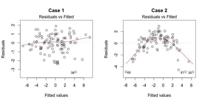
If the residuals randomly placed along a line, like case 1, than we can believe the data already have strong linearity.

Solution for non-Linearity

we should consider non-linear transformation for the features or adding non-linear terms of the features, so that the mapping relationship can be expressed by the hypothesis in a linear form

3. Evaluation for Autocorrelation

Autocorrelation refer to that there is a dependent mode between the randomized error of each sample . That is, the \(\epsilon\) of different are correlated. This would lead to underestimate the real randomized error \(\epsilon\).

Usually, the Autocorrelation happen when there exists time-sequence factors.

Detection of Autocorrelation

1.Time-sequence Plot

A simple and direct way to recognized the time-sequence of \(\epsilon\). Draw a plot of \(\epsilon\) sorted by time:

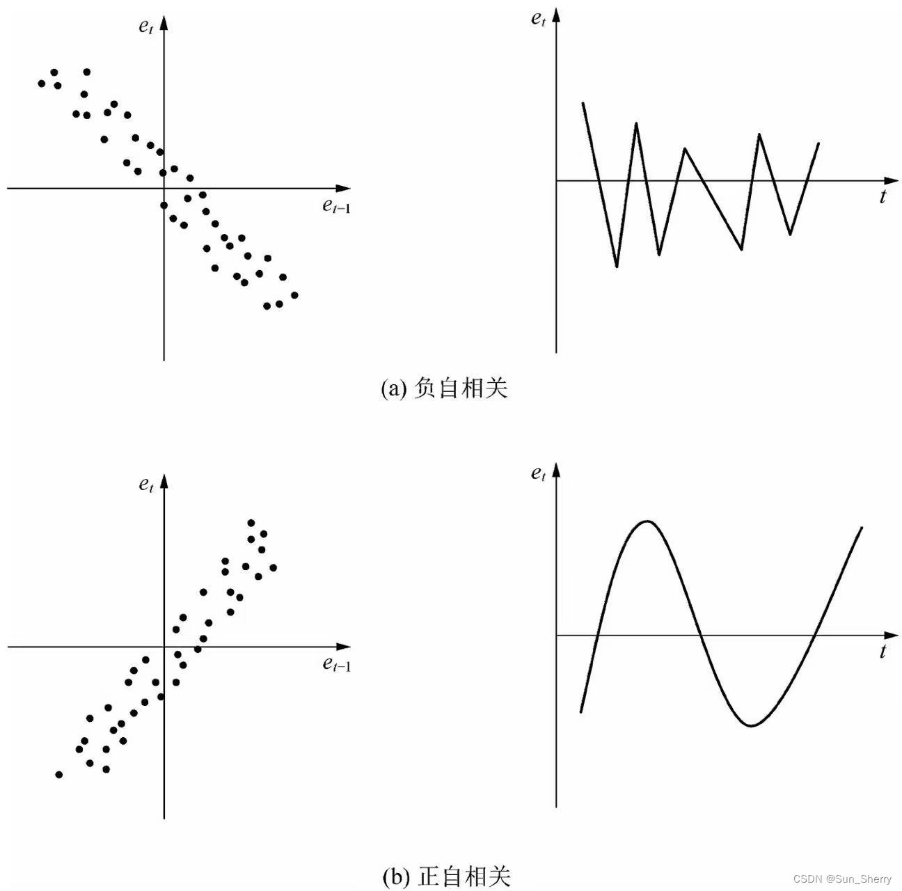
If the previous error \(e_{t-1}\) would make the next error \(e_t\) tend to be with opppsite sign, we call this a negative autocorrelation. Otherwise, we call it a positive autocorrelation.

2.DW Test

The DW test construct test statistics using the correction between \(e^{t-1}\) and \(e^t\). Gather errors of all sample and calculate \[ \rho = corr(e^t,e^{t-1}) \] Construct \[ DW \approx 2(1-\rho) \] according the Degree of Freedom n, we can look up in the table and find the upper bound and lower bound of the DW: \(d_U,d_L\), then we can examine which section the DW falls in to and make judgement on autocorrealtion:

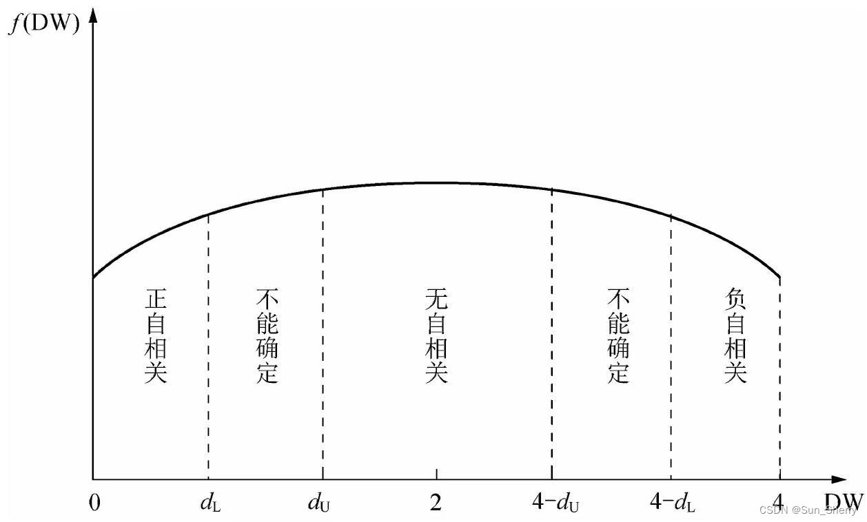
The drawbacks of DW test is that it has two uncertain sections. Besides, it cannot detect higher derivative autocorrelation than 1.

3.LM Test

It regress on $e^t $ with all feature X and lagged error \(e = e_{t-1},e_{t-2},..e_{t-p}\) with: \[ e_t = \alpha X + \rho e + \epsilon \] Where \(\rho\) is a vector, \(\rho_i\) is the correlation between \(e_t\) and \(e_{t-i}\). p is a hyperparameter for adjustment.

Obained the Judge coefficient \(R^2\) of the model, when sample size n is big, \((n-p)R^2 \sim \chi^2(p)\), we can than to a \(\chi^2\) test to examine whether there exist autocorrelation

Solution for Autocorrelation

The solution for autocorrelation:

• Consider time-sequence model
• If there exists positive autocorrelation, consider addling lagged feature \(X_{t-1},X_{t-2},...\) into the model
• If there exist seasonal factor, adding that factor into the model as dummies variable
• Generalized Difference Method: construct the model as:

\[ Y_t = \beta_0 + \beta_1X_t + \rho_1u_1+\rho_2u_2+...\rho_pu_p+\epsilon \]

Where \(u_i\) is the residual of the \(i^{th}\) model. This method has similar ideal like boosting. In machine learning, we can split the sample set into different moments according to timestamp like hour or date and construct serial models.

4. Evaluation of Multicollinearity

Multicollinearity refer to the relationship that a variable's change would cause another variable's change

In regression, we do not want there to be multicollinearity among input variables.

For example suppose we have a ideal regression model that \[ y = 10x_1+b \] Then we introduce a highly correlated variable \(x_2 = 2x_1\), in this case the modle can fit infinite possible combination of these two variables, for example, the model might end up with: \[ Y = -100x_1 +55x_2 +b = 10x_1+b \] These will cause:

• coefficient might lose its interpretability. Positive coefficient might turn negative, insignificant variable might turn significant
• The model might lose stability since the coefficients are enlarged. Small noises could cause big variance

Detection of Multicollinearity

1.Variance Inflation Factor \[ VIF_i=\frac{1}{1-R^ 2_i } \] The Variance Inflation Factor of the \(i^{th}\) variable \(X_i\) is the given by the Coefficient of Determination when regressing \(X_i\) with the rest m-1 variables.

In practice, if VIF > 10, we can consider as there's a Multicollinearity problem. If VIF > 100, we can consider as there's a serious Multicollinearity problem

2.Correlation Matrix

VIF demands large scale of calculation when the dimension of feature is high. A simpler way is to calculate the corrections matrixs using parameters like Pearson'r, Spearman'\(\rho\) or Kendall's \(\tau\)

Solution for Multicollinearity

The solution for Multicollinearity includes:

• Filtering feature selection methods based on correlation

• Wrapper feature engineering methods like stepwise regression

• Embedded Feature Engineering methods like Lasso & Ridge Regression

5. Evaluation for Homoskedasticity

Linear Regression Models require the variances of randomized to have same variance on different scale. That is, with the linearity assumption fulfilled, the variance of the model should be similar no matter how big the output variable is.

Detection of Heteroskedasticity

To detect heteroskedasticity, we can use Residual - Fitted Plot as well

In a RF plot, if the linearity assumption is satisfied, the point will place aside a horizontal line. If the model us biased, they would place around a leaned line or a curve. We call this line or curve the central line.

If the homoskedasticity is fulfilled, then the average distance from the point to the central line should be same across the axis of fitted values. If the errors has heteroskedasticity, then the points would be a shape like a spraying.

Solution for Heteroskedasticity

The solution for heteroskedasticity includes:

• Outlier detection: heteroskedasticity is usually caused by outliers.
• Distribution transformation on Y: heteroskedasticity can also be caused by the distribution of Y. Linear models require Y to be normally distributed. We can conduct distribution type transformation

6. Evaluation on Normality of \(\epsilon\)

The linear regression model requires the randomized error to be normally distributed. For normality test and normal transformation techniques, refer to this article